|
|
| Line 1: |
Line 1: |
| − | ==1,2,3-Trichloropropane (TCP)== | + | ==Estimating PCE/TCE Abiotic First-Order Reductive Dechlorination Rate Constants in Clayey Soils Under Anoxic Conditions== |
| − | [[Wikipedia: 1,2,3-Trichloropropane | 1,2,3-Trichloropropane (TCP)]] is a chlorinated volatile organic compound (CVOC) that has been used in chemical production processes, in agriculture, and as a solvent, resulting in point and non-point source contamination of soil and groundwater. TCP is mobile and highly persistent in soil and groundwater. TCP is not currently regulated at the national level in the United States, but [[Wikipedia: Maximum contaminant level | maximum contaminant levels (MCLs)]] have been developed by some states. Current treatment methods for TCP are limited and can be cost prohibitive. However, some treatment approaches, particularly [[Chemical Reduction (In Situ - ISCR) | ''in situ'' chemical reduction (ISCR)]] with [[Wikipedia: In_situ_chemical_reduction#Zero_valent_metals_%28ZVMs%29 | zero valent zinc (ZVZ)]] and [[Bioremediation - Anaerobic | ''in situ'' bioremediation (ISB)]], have recently been shown to have potential as practical remedies for TCP contamination of groundwater.
| + | The U.S. Department of Defense (DoD) faces many challenges in restoring aquifers at contaminated sites, often due to back-diffusion of tetrachloroethene (PCE) and trichloroethene (TCE) from low-permeability clay zones. The uptake, storage, and subsequent long-term release of these dissolved contaminants from clays are key processes in understanding the longevity, intensity, and risks associated with many persistent chlorinated ethene groundwater plumes. Although naturally occurring abiotic and biotic dechlorination processes in clays may reduce stored contaminant mass and significantly aid natural attenuation, no standardized field method currently exists to verify or quantify these reactions. It is critical to remediation design efforts to demonstrate and validate a cost-effective in situ approach for assessing these dechlorination processes using first-order rate constants. An approach was developed and applied across eight DoD sites to support Remedial Project Managers (RPMs) and regulators in evaluating natural attenuation potential in clay-rich environments. |
| | <div style="float:right;margin:0 0 2em 2em;">__TOC__</div> | | <div style="float:right;margin:0 0 2em 2em;">__TOC__</div> |
| | | | |
| | '''Related Article(s):''' | | '''Related Article(s):''' |
| − | *[[Bioremediation - Anaerobic | Anaerobic Bioremediation]]
| |
| − | *[[Chemical Reduction (In Situ - ISCR) | ''In Situ'' Chemical Reduction (ISCR)]]
| |
| − | *[[Chemical Oxidation (In Situ - ISCO) | ''In Situ'' Chemical Oxidation (ISCO)]]
| |
| | | | |
| − | '''Contributor(s):'''
| + | *[[Monitored Natural Attenuation (MNA)]] |
| − | *[[Dr. Alexandra Salter-Blanc | Alexandra J. Salter-Blanc]] | + | *[[Monitored Natural Attenuation (MNA) of Chlorinated Solvents]] |
| − | *[[Dr. Paul Tratnyek | Paul G. Tratnyek]] | + | *[[Monitored Natural Attenuation - Transitioning from Active Remedies]] |
| − | *John Merrill | + | *[[Matrix Diffusion]] |
| − | *Alyssa Saito
| + | *[[REMChlor - MD]] |
| − | *Lea Kane
| |
| − | *Eric Suchomel
| |
| − | *[[Dr. Rula Deeb | Rula Deeb]] | |
| | | | |
| − | '''Key Resource(s):''' | + | '''Contributors:''' Dani Tran, Dr. Charles Schaefer, Dr. Charles Werth |
| − | *Prospects for Remediation of 1,2,3-Trichloropropane by Natural and Engineered Abiotic Degradation Reactions. Strategic Environmental Research and Development Program (SERDP), Project ER-1457.<ref name="Tratnyek2010">Tratnyek, P.G., Sarathy, V., Salter, A.J., Nurmi, J.T., O’Brien Johnson, G., DeVoe, T., and Lee, P., 2010. Prospects for Remediation of 1,2,3-Trichloropropane by Natural and Engineered Abiotic Degradation Reactions. Strategic Environmental Research and Development Program (SERDP), Project ER-1457. [https://serdp-estcp.org/Program-Areas/Environmental-Restoration/Contaminated-Groundwater/Emerging-Issues/ER-1457/ER-1457/(language)/eng-US Website] [[Media: ER-1457-FR.pdf | Report.pdf]]</ref>
| |
| | | | |
| − | *Verification Monitoring for In Situ Chemical Reduction Using Zero-Valent Zinc, A Novel Technology for Remediation of Chlorinated Alkanes. Strategic Environmental Research and Development Program (SERDP), Project ER-201628.<ref name="Kane2020">Kane, L.Z., Suchomel, E.J., and Deeb, R.A., 2020. Verification Monitoring for In Situ Chemical Reduction Using Zero-Valent Zinc, A Novel Technology for Remediation of Chlorinated Alkanes. Strategic Environmental Research and Development Program (SERDP), Project ER-201628. [https://www.serdp-estcp.org/Program-Areas/Environmental-Restoration/Contaminated-Groundwater/Persistent-Contamination/ER-201628 Website] [[Media: ER-201628.pdf | Report.pdf]]</ref> | + | '''Key Resource:''' |
| | + | *Schaefer, C.E, Tran, D., Nguyen, D., Latta, D.E., Werth, C.J., 2025. Evaluating Mineral and In Situ Indicators of Abiotic Dechlorination in Clayey Soils<ref name="SchaeferEtAl2025"/> |
| | | | |
| | ==Introduction== | | ==Introduction== |
| − | [[File:123TCPFig1.png|thumb|left|Figure 1. Ball and stick representation of the molecular structure of TCP (Salter-Blanc and Tratnyek, unpublished)]]
| + | Cost-effective methods are needed to verify the occurrence of natural dechlorination processes and quantify their dechlorination rates in clays under ambient in situ conditions in order to reliably predict their long-term influence on plume longevity and mass discharge. However, accurately determining these rates is challenging due to slow reaction kinetics, the transient nature of transformation products, and the interplay of biotic and abiotic mechanisms within the clay matrix or at clay-sand interfaces. Tools capable of quantifying these reactions and assessing their role in mitigating plume persistence would be a significant aid for long-term site management. |
| − | 1,2,3-Trichloropropane (TCP) (Figure 1) is a man-made chemical that was used in the past primarily as a solvent and extractive agent, as a paint and varnish remover, and as a cleaning and degreasing agent.<ref name="ATSDR2021"> Agency for Toxic Substances and Disease Registry (ATSDR), 2021. Toxicological Profile for 1,2,3-Trichloropropane. Free download from: [https://www.atsdr.cdc.gov/toxprofiles/tp57.pdf ATSDR] [[Media: TCP2021ATSDR.pdf | Report.pdf]]</ref>. Currently, TCP is primarily used in chemical synthesis of compounds such as [[Wikipedia: Polysulfone | polysulfone]] liquid polymers used in the aerospace and automotive industries; [[Wikipedia: Hexafluoropropylene | hexafluoropropylene]] used in the agricultural, electronic, and pharmaceutical industries; [[Wikipedia: Polysulfide | polysulfide]] polymers used as sealants in manufacturing and construction; and [[Wikipedia: 1,3-Dichloropropene | 1,3-dichloropropene]] used in agriculture as a soil fumigant. TCP may also be present in products containing these chemicals as an impurity<ref name="ATSDR2021"/><ref name="CH2M2005">CH2M HILL, 2005. Interim Guidance for Investigating Potential 1,2,3-Trichloropropane Sources in San Gabriel Valley Area 3. [[Media: INTERIM_GUIDANCE_FOR_INVESTIGATING_POTENTIAL_1%2C2%2C3-TRICHLOROPROPANE_SOURCES.pdf | Report.pdf]] [https://cumulis.epa.gov/supercpad/cursites/csitinfo.cfm?id=0902093 Website]</ref>. For example, the 1,2-dichlropropane/1,3-dichloropropene soil fumigant mixture (trade name D-D), which is no longer sold in the United States, contained TCP as an impurity and has been linked to TCP contamination in groundwater<ref name="OkiGiambelluca1987">Oki, D.S. and Giambelluca, T.W., 1987. DBCP, EDB, and TCP Contamination of Ground Water in Hawaii. Groundwater, 25(6), pp. 693-702. [https://doi.org/10.1111/j.1745-6584.1987.tb02210.x DOI: 10.1111/j.1745-6584.1987.tb02210.x]</ref><ref name="CH2M2005"/>. Soil fumigants currently in use which are composed primarily of 1,3-dichloropropene may also contain TCP as an impurity, for instance Telone II has been reported to contain up to 0.17 percent TCP by weight<ref name="Kielhorn2003">Kielhorn, J., Könnecker, G., Pohlenz-Michel, C., Schmidt, S. and Mangelsdorf, I., 2003. Concise International Chemical Assessment Document 56: 1,2,3-Trichloropropane. World Health Organization, Geneva. [http://www.who.int/ipcs/publications/cicad/en/cicad56.pdf Website] [[Media: WHOcicad56TCP.pdf | Report.pdf]]</ref>.
| |
| | | | |
| − | TCP contamination is problematic because it is “reasonably anticipated to be a human carcinogen” based on evidence of carcinogenicity to animals<ref name="NTP2016"> National Toxicology Program, 2016. Report on Carcinogens, 14th ed. U.S. Department of Health and Human Services, Public Health Service. Free download from: [https://ntp.niehs.nih.gov/ntp/roc/content/profiles/trichloropropane.pdf NIH] [[Media: NTP2016trichloropropane.pdf | Report.pdf]]</ref>. Toxicity to humans appears to be high relative to other chlorinated solvents<ref name="Kielhorn2003"/>, suggesting that even low-level exposure to TCP could pose a significant human health risk.
| + | For reductive abiotic dechlorination under anoxic conditions, a 1% hydrochloric acid (HCl) extraction of a sample of native clay coupled with X-ray diffraction (XRD) data can be used as a screening level tool to estimate reductive dechlorination rate constants. These rate constants can be inserted into fate and transport models such as [[REMChlor - MD]]<ref>Falta, R., and Wang, W., 2017. A semi-analytical method for simulating matrix diffusion in numerical transport models. Journal of Contaminant Hydrology, 197, pp. 39-49. [https://doi.org/10.1016/j.jconhyd.2016.12.007 doi: 10.1016/j.jconhyd.2016.12.007] [[Media: FaltaWang2017.pdf | Open Access Manuscript]]</ref><ref>Kulkarni, P.R., Adamson, D.T., Popovic, J., Newell, C.J., 2022. Modeling a well-charactized perfluorooctane sulfate (PFOS) source and plume using the REMChlor-MD model to account for matrix diffusion. Journal of Contaminant Hydrology, 247, Article 103986. [https://doi.org/10.1016/j.jconhyd.2022.103986 doi: 10.1016/j.jconhyd.2022.103986] [[Media: KulkarniEtAl2022.pdf | Open Access Manuscript]]</ref> to quantify abiotic dechlorination impacts within clay aquitards on chlorinated solvent plumes. Thus, determination of the abiotic reductive dechlorination rate constant for a particular clayey soil can be readily utilized to provide a more accurate assessment of aquifer cleanup timeframes for groundwater plumes that are being sustained by contaminant back-diffusion. |
| | | | |
| − | ==Environmental Fate== | + | ==Recommended Approach== |
| − | TCP’s fate in the environment is governed by its physical and chemical properties (Table 1). TCP does not adsorb strongly to soil, making it likely to leach into groundwater and exhibit high mobility. In addition, TCP is moderately volatile and can partition from surface water and moist soil into the atmosphere. Because TCP is only slightly soluble and denser than water, it can form a [[Wikipedia: Dense non-aqueous phase liquid | dense non-aqueous phase liquid (DNAPL)]] as observed at the Tyson’s Dump Superfund Site<ref name="USEPA2019"> United States Environmental Protection Agency (USEPA), 2019. Fifth Five-year Review Report, Tyson’s Dump Superfund Site, Upper Merion Township, Montgomery County, Pennsylvania. Free download from: [https://semspub.epa.gov/work/03/2282817.pdf USEPA] [[Media: USEPA2019.pdf | Report.pdf]]</ref>. TCP is generally resistant to aerobic biodegradation, hydrolysis, oxidation, and reduction under naturally occurring conditions making it persistent in the environment<ref name="Tratnyek2010"/>.
| + | [[File: TranFig1.png | thumb | 500 px | Figure 1: First-order rate constants for abiotic reductive dechlorination of TCE under anaerobic conditions. Circles are data from Schaefer ''et al.'', 2021<ref>Schaefer, C.E., Ho, P., Berns, E., Werth, C., 2021. Abiotic dechlorination in the presence of ferrous minerals. Journal of Contaminant Hydrology, 241, 103839. [https://doi.org/10.1016/j.jconhyd.2021.103839 doi: 10.1016/j.jconhyd.2021.103839] [[Media: SchaeferEtAl2021.pdf | Open Access Manuscript]]</ref>, filled squares from Schaefer ''et al.'', 2018<ref name="SchaeferEtAl2018"/>, and Schaefer ''et al.'', 2017<ref>Schaefer, C.E., Ho., Gurr, C., Berns, E., Werth, C., 2017. Abiotic dechlorination of chlorinated ethenes in natural clayey soils: impacts of mineralogy and temperature. Journal of Contaminant Hydrology, 206, pp. 10-17. [https://doi.org/10.1016/j.jconhyd.2017.09.007 doi: 10.1016/j.jconhyd.2017.09.007] [[Media: SchaeferEtAl2017.pdf | Open Access Manuscript]]</ref>, and open squares from Schaefer ''et al.'', 2025<ref name="SchaeferEtAl2025"/>. ]] |
| | + | [[File: TranFig2.png | thumb | 600 px | Figure 2: Flowchart diagram of field screening procedures]] |
| | + | The recommended approach builds upon the methodology and findings of a recent study<ref name="SchaeferEtAl2025">Schaefer, C.E., Tran, D., Nguyen, D., Latta, D.E., Werth, C.J., 2025. Evaluating Mineral and In Situ Indicators of Abiotic Dechlorination in Clayey Soils. Groundwater Monitoring and Remediation, 45(2), pp. 31-39. [https://doi.org/10.1111/gwmr.12709 doi: 10.1111/gwmr.12709]</ref>, emphasizing field-based and analytical techniques to quantify abiotic first-order reductive dechlorination rate constants for PCE and TCE in clayey soils under anoxic conditions. Key components of this evaluation are listed below: |
| | + | #<u>Zone Identification:</u> The focus of the investigation should be to delineate clayey zones adjacent to hydraulically conductive zones. |
| | + | #<u>Ferrous Mineral Quantification:</u> Assess ferrous mineral context in clay via 1% HCl extraction at ambient temperature over a 10-minute interval. |
| | + | #<u>Mineralogical Characterization:</u> Conduct XRD analysis with the specific intent of identifying the presence of pyrite and biotite. |
| | + | #<u>Reduced Gas Analysis:</u> Measurement of reduced gases such as acetylene, ethene, and ethane concentrations in clay samples. Gas-tight sampling devices (e.g., En Core® soil samplers by En Novative Technologies, Inc.) should be used to ensure sample integrity during collection and transport. |
| | | | |
| − | {| class="wikitable" style="float:right; margin-left:10px;text-align:center;"
| + | Clay samples should be collected within a few centimeters of the high-permeability interface, with optional additional sampling further inward. For mineralogical analysis, a defined interval may be collected and subsequently subsampled. To preserve sample integrity, exposure to air should be minimized during collection, transport, and handling. Homogenization should occur within an anaerobic chamber, and if subsamples are required for external analysis, they must be shipped in gas-tight, anaerobic containers. |
| − | |+Table 1. Physical and chemical properties of TCP<ref name="USEPA2017">United States Environmental Protection Agency (USEPA), 2017. Technical Fact Sheet—1,2,3-Trichloropropane (TCP). EPA Project 505-F-17-007. 6 pp. Free download from: [https://www.epa.gov/sites/production/files/2017-10/documents/ffrrofactsheet_contaminants_tcp_9-15-17_508.pdf USEPA] [[Media: epa_tcp_2017.pdf | Report.pdf]]</ref>
| |
| − | |-
| |
| − | !Property
| |
| − | !Value
| |
| − | |-
| |
| − | | Chemical Abstracts Service (CAS) Number || 96-18-4
| |
| − | |-
| |
| − | | Physical Description</br>(at room temperature) || Colorless to straw-colored liquid
| |
| − | |-
| |
| − | | Molecular weight</br>(g/mol) || 147.43
| |
| − | |-
| |
| − | | Water solubility at 25°C</br>(mg/L)|| 1,750 (slightly soluble)
| |
| − | |-
| |
| − | | Melting point</br>(°C)|| -14.7
| |
| − | |-
| |
| − | | Boiling point</br>(°C) || 156.8
| |
| − | |-
| |
| − | | Vapor pressure at 25°C</br>(mm Hg) || 3.10 to 3.69
| |
| − | |-
| |
| − | | Density at 20°C (g/cm<sup>3</sup>) || 1.3889
| |
| − | |-
| |
| − | | Octanol-water partition coefficient</br>(log''K<sub>ow</sub>'') || 1.98 to 2.27</br>(temperature dependent)
| |
| − | |-
| |
| − | | Organic carbon-water partition coefficient</br>(log''K<sub>oc</sub>'') || 1.70 to 1.99</br>(temperature dependent)
| |
| − | |-
| |
| − | | Henry’s Law constant at 25°C</br>(atm-m<sup>3</sup>/mol) || 3.17x10<sup>-4</sup><ref name="ATSDR2021"/> to 3.43x10<sup>-4</sup><ref name="LeightonCalo1981">Leighton Jr, D.T. and Calo, J.M., 1981. Distribution Coefficients of Chlorinated Hydrocarbons in Dilute Air-Water Systems for Groundwater Contamination Applications. Journal of Chemical and Engineering Data, 26(4), pp. 382-385. [https://doi.org/10.1021/je00026a010 DOI: 10.1021/je00026a010]</ref>
| |
| − | |}
| |
| | | | |
| − | ==Occurrence==
| + | Estimation of the abiotic reductive first-order rate constant for PCE and TCE is based on the “reactive” ferrous content in the clay. Reactive ferrous content (Fe(II)<sub>r</sub>) is estimated as shown in Equation 1: |
| − | TCP has been detected in approximately 1% of public water supply and domestic well samples tested by the United States Geological Survey. More specifically, TCP was detected in 1.2% of public supply well samples collected between 1993 and 2007 by Toccalino and Hopple<ref name="ToccalinoHopple2010">Toccalino, P.L., Norman, J.E., Hitt, K.J., 2010. Quality of Source Water from Public-Supply Wells in the United States, 1993–2007. Scientific Investigations Report 2010-5024. U.S. Geological Survey. [https://doi.org/10.3133/sir20105024 DOI: 10.3133/sir20105024] Free download from: [https://pubs.er.usgs.gov/publication/sir20105024 USGS] [[Media: Quality_of_source_water_from_public-supply_wells_in_the_United_States%2C_1993-2007.pdf | Report.pdf]]</ref> and 0.66% of domestic supply well samples collected between 1991 and 2004 by DeSimone<ref name="DeSimone2009">DeSimone, L.A., 2009. Quality of Water from Domestic Wells in Principal Aquifers of the United States, 1991–2004. U.S. Geological Survey, Scientific Investigations Report 2008–5227. 139 pp. Free download from: [http://pubs.usgs.gov/sir/2008/5227 USGS] [[Media: DeSimone2009.pdf | Report.pdf]]</ref>. TCP was detected at a higher rate in domestic supply well samples associated with agricultural land-use studies than samples associated with studies comparing primary aquifers (3.5% versus 0.2%)<ref name="DeSimone2009"/>.
| |
| | | | |
| − | ==Regulation==
| + | ::'''Equation 1:''' <big>''Fe(II)<sub><small>r</small></sub> = DA + XRD<sub><small>pyr</small></sub> - XRD<sub><small>biotite</small></sub>''</big> |
| − | The United States Environmental Protection Agency (USEPA) has not established an MCL for TCP, although guidelines and health standards are in place<ref name="USEPA2017"/>. TCP was included in the Contaminant Candidate List 3<ref name="USEPA2009">United States Environmental Protection Agency (US EPA), 2009. Drinking Water Contaminant Candidate List 3-Final. Federal Register 74(194), pp. 51850–51862, Document E9-24287. [https://www.federalregister.gov/documents/2009/10/08/E9-24287/drinking-water-contaminant-candidate-list-3-final Website] [[Media: FR74-194DWCCL3.pdf | Report.pdf]]</ref> and the Unregulated Contaminant Monitoring Rule 3 (UCMR 3)<ref name="USEPA2012">United States Environmental Protection Agency (US EPA), 2012. Revisions to the Unregulated Contaminant Mentoring Regulation (UCMR 3) for Public Water Systems. Federal Register 77(85) pp. 26072-26101. [https://www.federalregister.gov/documents/2012/05/02/2012-9978/revisions-to-the-unregulated-contaminant-monitoring-regulation-ucmr-3-for-public-water-systems Website] [[Media: FR77-85UCMR3.pdf | Report.pdf]]</ref>. The UCMR 3 specified that data be collected on TCP occurrence in public water systems over the period of January 2013 through December 2015 against a reference concentration range of 0.0004 to 0.04 μg/L<ref name="USEPA2017a">United States Environmental Protection Agency (USEPA), 2017. The Third Unregulated Contaminant Monitoring Rule (UCMR 3): Data Summary. EPA 815-S-17-001. [https://www.epa.gov/dwucmr/data-summary-third-unregulated-contaminant-monitoring-rule Website] [[Media: ucmr3-data-summary-january-2017.pdf | Report.pdf]]</ref>. The reference concentration range was determined based on a cancer risk of 10-6 to 10-4 and derived from an oral slope factor of 30 mg/kg-day, which was determined by the EPA’s Integrated Risk Information System<ref name="IRIS2009">USEPA Integrated Risk Information System (IRIS), 2009. 1,2,3-Trichloropropane (CASRN 96-18-4). [https://cfpub.epa.gov/ncea/iris2/chemicalLanding.cfm?substance_nmbr=200 Website] [[Media: TCPsummaryIRIS.pdf | Summary.pdf]]</ref>. Of 36,848 samples collected during UCMR 3, 0.67% exceeded the minimum reporting level of 0.03 µg/L. 1.4% of public water systems had at least one detection over the minimum reporting level, corresponding to 2.5% of the population<ref name="USEPA2017a"/>. While these occurrence percentages are relatively low, the minimum reporting level of 0.03 µg/L is more than 75 times the USEPA-calculated Health Reference Level of 0.0004 µg/L. Because of this, TCP may occur in public water systems at concentrations that exceed the Health Reference Level but are below the minimum reporting level used during UCMR 3 data collection. These analytical limitations and lack of lower-level occurrence data have prevented the USEPA from making a preliminary regulatory determination for TCP<ref name="USEPA2021">USEPA, 2021. Announcement of Final Regulatory Determinations for Contaminants on the Fourth Drinking Water Contaminant Candidate List. Free download from: [https://www.epa.gov/sites/default/files/2021-01/documents/10019.70.ow_ccl_reg_det_4.final_web.pdf USEPA] [[Media: CCL4.pdf | Report.pdf]]</ref>.
| |
| | | | |
| − | Some US states have established their own standards including Hawaii which has established an MCL of 0.6 μg/L<ref name="HDOH2013">Hawaii Department of Health, 2013. Amendment and Compilation of Chapter 11-20 Hawaii Administrative Rules. Free download from: [http://health.hawaii.gov/sdwb/files/2016/06/combodOPPPD.pdf Hawaii Department of Health] [[Media: Amendment_and_Compilation_of_Chapter_11-20_Hawaii_Administrative_Rules.pdf | Report.pdf]]</ref>. California has established an MCL of 0.005 μg/L<ref name="CCR2021">California Code of Regulations, 2021. Section 64444 Maximum Contaminant Levels – Organic Chemicals (22 CA ADC § 64444). [https://govt.westlaw.com/calregs/Document/IA7B3800D18654ABD9E2D24A445A66CB9 Website]</ref>, a notification level of 0.005 μg/L, and a public health goal of 0.0007 μg/L<ref name="OEHHA2009">Office of Environmental Health Hazard Assessment (OEHHA), California Environmental Protection Agency, 2009. Final Public Health Goal for 1,2,3-Trichloropropane in Drinking Water. [https://oehha.ca.gov/water/public-health-goal/final-public-health-goal-123-trichloropropane-drinking-water Website]</ref>, and New Jersey has established an MCL of 0.03 μg/L<ref name="NJAC2020">New Jersey Administrative Code 7:10, 2020. Safe Drinking Water Act Rules. Free download from: [https://www.nj.gov/dep/rules/rules/njac7_10.pdf New Jersey Department of Environmental Protection]</ref>.
| + | where ''DA'' is the ferrous content from the dilute acid (1% HCl) extraction, ''XRD<sub><small>pyr</small></sub>'' is the pyrite content from XRD analysis, and ''XRD<sub><small>biotite</small></sub>'' is the biotite content from XRD analysis<ref name="SchaeferEtAl2025"/>. |
| | | | |
| − | ==Transformation Processes== | + | Abiotic dechlorination is unlikely to contribute to mitigating contaminant back-diffusion when reactive ferrous iron (Fe(II)<sub><small>r</small></sub>) concentrations are below 100 mg/kg (Figure 1). For Fe(II)<sub><small>r</small></sub> above 100 mg/kg, the first-order rate constant for PCE and TCE reductive dechlorination can be estimated using the correlation shown in Figure 1<ref name="SchaeferEtAl2018">Schaefer, C.E., Ho, P., Berns, E., Werth, C., 2018. Mechanisms for abiotic dechlorination of trichloroethene by ferrous minerals under oxic and anoxic conditions in natural sediments. Environmental Science and Technology, 52(23), pp.13747-13755. [https://doi.org/10.1021/acs.est.8b04108 doi: 10.1021/acs.est.8b04108]</ref><ref>Borden, R.C., Cha, K.Y., 2021. Evaluating the impact of back diffusion on groundwater cleanup time. Journal of Contaminant Hydrology, 243, Article 103889. [https://doi.org/10.1016/j.jconhyd.2021.103889 doi: 10.1016/j.jconhyd.2021] [[Media: BordenCha2021.pdf | Open Access Manuscript]]</ref>. The rate constant exhibits a strong positive correlation with the logarithm of reactive Fe(II) content (Pearson’s ''r'' = 0.82), with a slope of 4.7 × 10⁻⁸ L g⁻¹ d⁻¹ (log mg kg⁻¹)⁻¹. |
| | | | |
| | + | Figure 2 presents a decision flowchart designed to evaluate the significance and extent of abiotic reductive dechlorination. By applying Equation 1 to the dilute acid extractable Fe(II) plus measured mineral species data from clay samples, the reactive ferrous iron content (Fe(II)<sub><small>r</small></sub>) can be quantified, enabling a streamlined assessment of the extent to which abiotic processes are contributing to the mitigation of contaminant back-diffusion. |
| | | | |
| − | {| class="wikitable" style="float:right; margin-left:10px;text-align:center;"
| + | If Fe(II)r is ≥ 100 mg/kg, a first-order dechlorination rate constant can be estimated and subsequently used within a contaminant fate and transport model. However, if acetylene is detected in the clay, even with Fe(II)r less than 100 mg/kg, then bench-scale testing using methods similar to those described in a recent study<ref name="SchaeferEtAl2025"/> is recommended, as such results would likely be inconsistent with those shown in Figure 1, suggesting some other mechanism might be involved, or that the system mineralogy might be more complex than anticipated. Even if Fe(II)r ≥ 100 mg/kg, confirmatory bench-scale testing may be conducted for additional verification and to refine estimation of the abiotic dechlorination rate constant. |
| − | |+Table 2. Advantages and limitations of TCP treatment technologies
| |
| − | |-
| |
| − | ! Technology
| |
| − | ! Advantages
| |
| − | ! Limitations
| |
| − | |-
| |
| − | | ZVZ
| |
| − | | style="text-align:left;" |
| |
| − | * Can degrade TCP at relatively high and low concentrations
| |
| − | * Faster reaction rates than ZVI
| |
| − | * Material is commercially available
| |
| − | | style="text-align:left;" |
| |
| − | * Higher cost than ZVI
| |
| − | * Difficult to distribute in subsurface ''in situ'' applications
| |
| − | |-
| |
| − | | Groundwater</br>Extraction and</br>Treatment
| |
| − | | style="text-align:left;" |
| |
| − | * Can cost-effectively capture and treat larger, more dilute</br>groundwater plumes than ''in situ'' technologies
| |
| − | * Well understood and widely applied technology
| |
| − | | style="text-align:left;" |
| |
| − | * Requires construction, operation and maintenance of</br>aboveground treatment infrastructure
| |
| − | * Typical technologies (e.g. GAC) may be expensive due</br>to treatment inefficiencies
| |
| − | |-
| |
| − | | ZVI
| |
| − | | style="text-align:left;" |
| |
| − | * Can degrade TCP at relatively high and low concentrations
| |
| − | * Lower cost than ZVZ
| |
| − | * Material is commercially available
| |
| − | | style="text-align:left;" |
| |
| − | * Lower reactivity than ZVZ, therefore may require higher</br>ZVI volumes or thicker PRBs
| |
| − | * Difficult to distribute in subsurface ''in situ'' applications
| |
| − | |-
| |
| − | | ISCO
| |
| − | | style="text-align:left;" |
| |
| − | * Can degrade TCP at relatively high and low concentrations
| |
| − | * Strategies to distribute amendments ''in situ'' are well established
| |
| − | * Material is commercially available
| |
| − | | style="text-align:left;" |
| |
| − | * Most effective oxidants (e.g., base-activated or heat-activated</br>persulfate) are complex to implement
| |
| − | * Secondary water quality impacts (e.g., high pH, sulfate, </br>hexavalent chromium) may limit ability to implement
| |
| − | |-
| |
| − | | ''In Situ''</br>Bioremediation
| |
| − | | style="text-align:left;" |
| |
| − | * Can degrade TCP at moderate to high concentrations
| |
| − | * Strategies to distribute amendments ''in situ'' are well established
| |
| − | * Materials are commercially available and inexpensive
| |
| − | | style="text-align:left;" |
| |
| − | * Slower reaction rates than ZVZ or ISCO
| |
| − | |}
| |
| | | | |
| | + | ==Summary and Recommendations== |
| | + | The approach outlined above is intended to serve as a generalized guide for practitioners and site managers to cost-effectively determine the extent to which beneficial abiotic reductive dechlorination reactions are likely occurring in low permeability (e.g., clayey) zones. This approach may be contraindicated if co-contaminants are present. It is currently unclear whether other classes of potentially reactive chemicals, such as trinitrotoluene (TNT) or chlorinated ethanes, could interact competitively with PCE and TCE. |
| | | | |
| | + | In addition, it remains unclear how other classes of compounds such as per- and polyfluoroalkyl substances (PFAS) may interact or sorb with ferrous minerals and potentially inhibit abiotic dechlorination reactions. Coupling these recommended activities with conventional site investigation tasks would provide an opportunity to perform many of the up-front screening activities with minimal additional project costs. It is important to note that the guidance proposed herein pertains to particularly low permeability media. Sites with complex or varying lithology, where the mineralogy and/or redox conditions may vary, might require evaluation of multiple samples to provide appropriate site-wide information. |
| | | | |
| − | There are two main approaches to downscaling. One method, commonly referred to as “statistical downscaling”, uses the empirical-statistical relationships between large-scale weather phenomena and historical local weather data. In this method, these statistical relationships are applied to output generated by global climate models. A second method uses physics-based numerical models (regional-scale climate models or RCMs) of weather and climate that operate over a limited region of the earth (e.g., North America) and at spatial resolutions that are typically 3 to 10 times finer than the global-scale climate models. This method is known as “dynamical downscaling”. These regional-scale climate models are similar to the global models with respect to their reliance on the principles of physics, but because they operate over only part of the earth, they require information about what is coming in from the rest of the earth as well as what is going out of the limited region of the model. This is generally obtained from a global model. The primary differences between statistical and dynamical downscaling methods are summarized in Table 1.
| + | <br clear="right"/> |
| − | | |
| − | It is important to realize that there is no “best” downscaling method or dataset, and that the best method/dataset for a given problem depends on that problem’s specific needs. Several data products based on downscaling higher level spatial data are available ([https://cida.usgs.gov/gdp/ USGS], [http://maca.northwestknowledge.net/ MACA], [https://www.narccap.ucar.edu/ NARCCAP], [https://na-cordex.org/ CORDEX-NA]). The appropriate method and dataset to use depends on the intended application. The method selected should be able to credibly resolve spatial and temporal scales relevant for the application. For example, to develop a risk analysis of frequent flooding, the data product chosen should include precipitation at greater than a diurnal frequency and over multi-decadal timescales. This kind of product is most likely to be available using the dynamical downscaling method. SERDP reviewed the various advantages and disadvantages of using each type of downscaling method and downscaling dataset, and developed a recommended process that is publicly available<ref name="Kotamarthi2016"/>. In general, the following recommendations should be considered in order to pick the right downscaled dataset for a given analysis:
| |
| − | | |
| − | * When a problem depends on using a large number of climate models and emission scenarios to perform preliminary assessments and to understand the uncertainty range of projections, then using a statistical downscaled dataset is recommended.
| |
| − | * When the assessment needs a more extensive parameter list or is analyzing a region with few long-term observational data, dynamically downscaled climate change projections are recommended.
| |
| − | | |
| − | ==Uncertainty in Projections==
| |
| − | {| class="wikitable" style="float:right; margin-left:10px;text-align:center;"
| |
| − | |+Table 2. Downscaling model characteristics and output<ref name="Kotamarthi2016"/>
| |
| − | |-
| |
| − | !Model or</br>Dataset Name
| |
| − | !Model<br />Method
| |
| − | !Output<br />Variables
| |
| − | !Output<br />Format
| |
| − | !Spatial</br>Resolution
| |
| − | !Time</br>Resolution
| |
| − | |-
| |
| − | | colspan="6" style="text-align: left; background-color:white;" |'''Statistical Downscaled Datasets'''
| |
| − | |-
| |
| − | | [https://worldclim.org/data/index.html WorldClim]<ref name="Hijmans2005">Hijmans, R.J., Cameron, S.E., Parra, J.L., Jones, P.G. and Jarvis, A., 2005. Very High Resolution Interpolated Climate Surfaces for Global Land Areas. International Journal of Climatology: A Journal of the Royal Meteorological Society, 25(15), pp 1965-1978. [https://doi.org/10.1002/joc.1276 DOI: 10.1002/joc.1276]</ref>
| |
| − | |Delta||T(min, max,</br>avg), Pr||NetCDF||grid: 30 arc sec to</br>10 arc min||month
| |
| − | |-
| |
| − | | Bias Corrected / Spatial</br>Disaggregation (BCSD)<ref name="Wood2002">Wood, A.W., Maurer, E.P., Kumar, A. and Lettenmaier, D.P., 2002. Long‐range experimental hydrologic forecasting for the eastern United States. Journal of Geophysical Research: Atmospheres, 107(D20), 4429, pp. ACL6 1-15. [https://doi.org/10.1029/2001JD000659 DOI:10.1029/2001JD000659] Free access article available from: [https://agupubs.onlinelibrary.wiley.com/doi/abs/10.1029/2001JD000659 American Geophysical Union] [[Media: Wood2002.pdf | Report.pdf ]]</ref>
| |
| − | |Empirical Quantile</br>Mapping||Runoff,</br>Streamflow||NetCDF||grid: 7.5 arc min||day
| |
| − | |-
| |
| − | | [https://cida.usgs.gov/thredds/catalog.html?dataset=dcp Asynchronous Regional Regression</br>Model (ARRM v.1)]<ref name="Stoner2013">Stoner, A.M., Hayhoe, K., Yang, X., and Wuebbles, D.J., 2013. An Asynchronous Regional Regression Model for Statistical Downscaling of Daily Climate Variables. International Journal of Climatology, 33(11), pp. 2473-2494. [https://doi.org/10.1002/joc.3603 DOI:10.1002/joc.3603]</ref>
| |
| − | |Parameterized</br>Quantile Mapping||T(min, max), Pr||NetCDF||stations plus</br>grid: 7.5 arc min||day
| |
| − | |-
| |
| − | | [https://sdsm.org.uk/ Statistical Downscaling Model (SDSM)]<ref name="Wilby2013">Wilby, R.L., and Dawson, C.W., 2013. The Statistical DownScaling Model: insights from one decade of application. International Journal of Climatology, 33(7), pp. 1707-1719. [https://doi.org/10.1002/joc.3544 DOI: 10.1002/joc.3544]</ref>
| |
| − | |Weather Generator||T(min, max), Pr||PC Code||stations||day
| |
| − | |-
| |
| − | | [https://climate.northwestknowledge.net/MACA/ Multivariate Adaptive</br>Constructed Analogs (MACA)]<ref name="Hidalgo2008">Hidalgo, H.G., Dettinger, M.D. and Cayan, D.R., 2008. Downscaling with Constructed Analogues: Daily Precipitation and Temperature Fields Over the United States. California Energy Commission PIER Final Project, Report CEC-500-2007-123. [[Media: Hidalgo2008.PDF | Report.pdf]]</ref>
| |
| − | |Constructed Analogues||10 Variables||NetCDF||grid: 2.5 arc min||day
| |
| − | |-
| |
| − | | [http://loca.ucsd.edu/ Localized Constructed Analogs (LOCA)]<ref name="Pierce2013">Pierce, D.W., Cayan, D.R. and Thrasher, B.L., 2014. Statistical Downscaling Using Localized Constructed Analogs (LOCA). Journal of Hydrometeorology, 15(6), pp. 2558-2585. [https://doi.org/10.1175/JHM-D-14-0082.1 DOI: 10.1175/JHM-D-14-0082.1] Free access article available from: [https://journals.ametsoc.org/view/journals/hydr/15/6/jhm-d-14-0082_1.xml American Meteorological Society]. [[Media: Pierce2014.pdf | Report.pdf]]</ref>
| |
| − | |Constructed Analogues||T(min, max), Pr||NetCDF||grid: 3.75 arc min||day
| |
| − | |-
| |
| − | | [https://www.nccs.nasa.gov/services/data-collections/land-based-products/nex-dcp30 NASA Earth Exchange Downscaled</br>Climate Projections (NEX-DCP30)]<ref name="Wood2002"/>
| |
| − | |Bias Correction /</br>Spatial Disaggregation||T(min, max), Pr||NetCDF||grid: 30 arc sec||month
| |
| − | |-
| |
| − | | colspan="6" style="text-align: left; background-color:white;" |'''Dynamical Downscaled Datasets'''
| |
| − | |-
| |
| − | | [http://www.narccap.ucar.edu/index.html North American Regional Climate</br>Change Assessment Program (NARCCAP)]<ref name="Mearns2009">Mearns, L.O., Gutowski, W., Jones, R., Leung, R., McGinnis, S., Nunes, A. and Qian, Y., 2009. A Regional Climate Change Assessment Program for North America. Eos, Transactions, American Geophysical Union, 90(36), p.311. [https://doi.org/10.1029/2009EO360002 DOI: 10.1029/2009EO360002] Free access article from: [https://agupubs.onlinelibrary.wiley.com/doi/abs/10.1029/2009EO360002 American Geophysical Union] [[Media: Mearns2009.pdf | Report.pdf]]</ref>
| |
| − | |Multiple Models||49 Variables||NetCDF||grid: 30 arc min||3 hours
| |
| − | |-
| |
| − | | [https://cordex.org/about/ Coordinated Regional Climate</br>Downscaling Experiment (CORDEX)]<ref name="Giorgi2009">Giorgi, F., Jones, C., and Asrar, G.R., 2009. Addressing climate information needs at the regional level: the CORDEX framework. World Meteorological Organization (WMO) Bulletin, 58(3), pp. 175-183. Free access article from: [https://public.wmo.int/en/bulletin/addressing-climate-information-needs-regional-level-cordex-framework World Meteorological Organization] [[Media: Giorgi2009.pdf | Report.pdf]]</ref>
| |
| − | |Multiple Models||66 Variables||NetCDF||grid: 30 arc min||3 hours
| |
| − | |-
| |
| − | | [https://esrl.noaa.gov/gsd/wrfportal/ Strategic Environmental Research and</br>Development Program (SERDP)]<ref name="Wang2015">Wang, J., and Kotamarthi, V.R., 2015. High‐resolution dynamically downscaled projections of precipitation in the mid and late 21st century over North America. Earth's Future, 3(7), pp. 268-288. [https://doi.org/10.1002/2015EF000304 DOI: 10.1002/2015EF000304] Free access article from: [https://agupubs.onlinelibrary.wiley.com/doi/full/10.1002/2015EF000304 American Geophysical Union] [[Media: Wang2015.pdf | Report.pdf]]</ref>
| |
| − | |Weather Research and</br>Forecasting (WRF v3.3)||80+ Variables||NetCDF||grid: 6.5 arc min||3 hours
| |
| − | |}
| |
| − | A primary cause of uncertainty in climate change projections, especially beyond 30 years into the future, is the uncertainty in the greenhouse gas (GHG) emission scenarios used to make climate model projections. The best method of accounting for this type of uncertainty is to apply a climate change model to multiple GHG emission scenarios (see also: [[Wikipedia: Representative Concentration Pathway]]).
| |
| − | | |
| − | The uncertainties in climate projections over shorter timescales, less than 30 years out, are dominated by something known as “internal variability” in the models. Different approaches are used to address the uncertainty from internal variability<ref name="Kotamarthi2021"/>. A third type of uncertainty in climate modeling, known as scientific uncertainty, comes from our inability to numerically solve every aspect of the complex earth system. We expect this scientific uncertainty to decrease as we understand more of the earth system and improve its representation in our numerical models. As discussed in [[Climate Change Primer]], numerical experiments based on global climate models are designed to address these uncertainties in various ways. Downscaling methods evaluate this uncertainty by using several independent regional climate models to generate future projections, with the expectation that each of these models will capture some aspects of the physics better than the others, and that by using several different models, we can estimate the range of this uncertainty. Thus, the commonly accepted methods for accounting for uncertainty in climate model projections are either using projections from one model for several emission scenarios, or applying multiple models to project a single scenario.
| |
| − | | |
| − | A comparison of the currently available methods and their characteristics is provided in Table 2 (adapted from Kotamarthi et al., 2016<ref name="Kotamarthi2016"/>). The table lists the various methodologies and models used for producing downscaled data, and the climate variables that these methods produce. These datasets are mostly available for download from the data servers and websites listed in the table and in a few cases by contacting the respective source organizations.
| |
| − | | |
| − | The most popular and widely used format for atmospheric and climate science is known as [[Wikipedia:NetCDF | NetCDF]], which stands for Network Common Data Form. NetCDF is a self-describing data format that saves data in a binary format. The format is self-describing in that a metadata listing is part of every file that describes all the data attributes, such as dimensions, units and data size and in principal should not need additional information to extract the required data for analysis with the right software. However, specially built software for reading and extracting data from these binary files is necessary for making visualizations and further analysis. Software packages for reading and writing NetCDF datasets and for generating visualizations from these datasets are widely available and obtained free of cost ([https://www.unidata.ucar.edu/software/netcdf/docs/ NetCDF-tools]). Popular geospatial analysis tools such as ARC-GIS, statistical packages such as ‘R’ and programming languages such as Fortran, C++, and Python have built in libraries that can be used to directly read NetCDF files for visualization and analysis.
| |
| − | <br clear="left" />
| |
| | | | |
| | ==References== | | ==References== |
| | <references /> | | <references /> |
| | + | |
| | ==See Also== | | ==See Also== |
| − | | + | *[https://serdp-estcp.mil/projects/details/a7e3f7b5-ed82-4591-adaa-6196ff33dd60 ESTCP Project ER20-5031 – In Situ Verification and Quantification of Naturally Occurring Dechlorination Rates in Clays: Demonstrating Processes that Mitigate Back-Diffusion and Plume Persistence] |
| − | [https://serdp-estcp.org/Program-Areas/Resource-Conservation-and-Resiliency/Infrastructure-Resiliency/Vulnerability-and-Impact-Assessment/RC-2242/(language)/eng-US Climate Change Impacts to Department of Defense Installations, SERDP Project RC-2242] | |
Estimating PCE/TCE Abiotic First-Order Reductive Dechlorination Rate Constants in Clayey Soils Under Anoxic Conditions
The U.S. Department of Defense (DoD) faces many challenges in restoring aquifers at contaminated sites, often due to back-diffusion of tetrachloroethene (PCE) and trichloroethene (TCE) from low-permeability clay zones. The uptake, storage, and subsequent long-term release of these dissolved contaminants from clays are key processes in understanding the longevity, intensity, and risks associated with many persistent chlorinated ethene groundwater plumes. Although naturally occurring abiotic and biotic dechlorination processes in clays may reduce stored contaminant mass and significantly aid natural attenuation, no standardized field method currently exists to verify or quantify these reactions. It is critical to remediation design efforts to demonstrate and validate a cost-effective in situ approach for assessing these dechlorination processes using first-order rate constants. An approach was developed and applied across eight DoD sites to support Remedial Project Managers (RPMs) and regulators in evaluating natural attenuation potential in clay-rich environments.
Related Article(s):
Contributors: Dani Tran, Dr. Charles Schaefer, Dr. Charles Werth
Key Resource:
- Schaefer, C.E, Tran, D., Nguyen, D., Latta, D.E., Werth, C.J., 2025. Evaluating Mineral and In Situ Indicators of Abiotic Dechlorination in Clayey Soils[1]
Introduction
Cost-effective methods are needed to verify the occurrence of natural dechlorination processes and quantify their dechlorination rates in clays under ambient in situ conditions in order to reliably predict their long-term influence on plume longevity and mass discharge. However, accurately determining these rates is challenging due to slow reaction kinetics, the transient nature of transformation products, and the interplay of biotic and abiotic mechanisms within the clay matrix or at clay-sand interfaces. Tools capable of quantifying these reactions and assessing their role in mitigating plume persistence would be a significant aid for long-term site management.
For reductive abiotic dechlorination under anoxic conditions, a 1% hydrochloric acid (HCl) extraction of a sample of native clay coupled with X-ray diffraction (XRD) data can be used as a screening level tool to estimate reductive dechlorination rate constants. These rate constants can be inserted into fate and transport models such as REMChlor - MD[2][3] to quantify abiotic dechlorination impacts within clay aquitards on chlorinated solvent plumes. Thus, determination of the abiotic reductive dechlorination rate constant for a particular clayey soil can be readily utilized to provide a more accurate assessment of aquifer cleanup timeframes for groundwater plumes that are being sustained by contaminant back-diffusion.
Recommended Approach
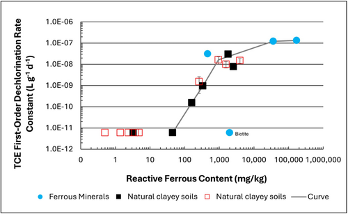
Figure 1: First-order rate constants for abiotic reductive dechlorination of TCE under anaerobic conditions. Circles are data from Schaefer
et al., 2021
[4], filled squares from Schaefer
et al., 2018
[5], and Schaefer
et al., 2017
[6], and open squares from Schaefer
et al., 2025
[1].
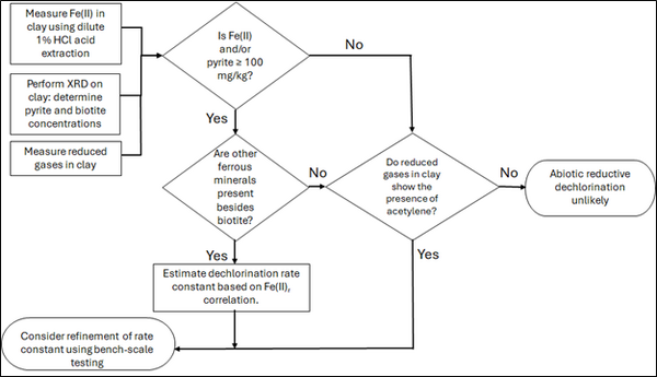
Figure 2: Flowchart diagram of field screening procedures
The recommended approach builds upon the methodology and findings of a recent study[1], emphasizing field-based and analytical techniques to quantify abiotic first-order reductive dechlorination rate constants for PCE and TCE in clayey soils under anoxic conditions. Key components of this evaluation are listed below:
- Zone Identification: The focus of the investigation should be to delineate clayey zones adjacent to hydraulically conductive zones.
- Ferrous Mineral Quantification: Assess ferrous mineral context in clay via 1% HCl extraction at ambient temperature over a 10-minute interval.
- Mineralogical Characterization: Conduct XRD analysis with the specific intent of identifying the presence of pyrite and biotite.
- Reduced Gas Analysis: Measurement of reduced gases such as acetylene, ethene, and ethane concentrations in clay samples. Gas-tight sampling devices (e.g., En Core® soil samplers by En Novative Technologies, Inc.) should be used to ensure sample integrity during collection and transport.
Clay samples should be collected within a few centimeters of the high-permeability interface, with optional additional sampling further inward. For mineralogical analysis, a defined interval may be collected and subsequently subsampled. To preserve sample integrity, exposure to air should be minimized during collection, transport, and handling. Homogenization should occur within an anaerobic chamber, and if subsamples are required for external analysis, they must be shipped in gas-tight, anaerobic containers.
Estimation of the abiotic reductive first-order rate constant for PCE and TCE is based on the “reactive” ferrous content in the clay. Reactive ferrous content (Fe(II)r) is estimated as shown in Equation 1:
- Equation 1: Fe(II)r = DA + XRDpyr - XRDbiotite
where DA is the ferrous content from the dilute acid (1% HCl) extraction, XRDpyr is the pyrite content from XRD analysis, and XRDbiotite is the biotite content from XRD analysis[1].
Abiotic dechlorination is unlikely to contribute to mitigating contaminant back-diffusion when reactive ferrous iron (Fe(II)r) concentrations are below 100 mg/kg (Figure 1). For Fe(II)r above 100 mg/kg, the first-order rate constant for PCE and TCE reductive dechlorination can be estimated using the correlation shown in Figure 1[5][7]. The rate constant exhibits a strong positive correlation with the logarithm of reactive Fe(II) content (Pearson’s r = 0.82), with a slope of 4.7 × 10⁻⁸ L g⁻¹ d⁻¹ (log mg kg⁻¹)⁻¹.
Figure 2 presents a decision flowchart designed to evaluate the significance and extent of abiotic reductive dechlorination. By applying Equation 1 to the dilute acid extractable Fe(II) plus measured mineral species data from clay samples, the reactive ferrous iron content (Fe(II)r) can be quantified, enabling a streamlined assessment of the extent to which abiotic processes are contributing to the mitigation of contaminant back-diffusion.
If Fe(II)r is ≥ 100 mg/kg, a first-order dechlorination rate constant can be estimated and subsequently used within a contaminant fate and transport model. However, if acetylene is detected in the clay, even with Fe(II)r less than 100 mg/kg, then bench-scale testing using methods similar to those described in a recent study[1] is recommended, as such results would likely be inconsistent with those shown in Figure 1, suggesting some other mechanism might be involved, or that the system mineralogy might be more complex than anticipated. Even if Fe(II)r ≥ 100 mg/kg, confirmatory bench-scale testing may be conducted for additional verification and to refine estimation of the abiotic dechlorination rate constant.
Summary and Recommendations
The approach outlined above is intended to serve as a generalized guide for practitioners and site managers to cost-effectively determine the extent to which beneficial abiotic reductive dechlorination reactions are likely occurring in low permeability (e.g., clayey) zones. This approach may be contraindicated if co-contaminants are present. It is currently unclear whether other classes of potentially reactive chemicals, such as trinitrotoluene (TNT) or chlorinated ethanes, could interact competitively with PCE and TCE.
In addition, it remains unclear how other classes of compounds such as per- and polyfluoroalkyl substances (PFAS) may interact or sorb with ferrous minerals and potentially inhibit abiotic dechlorination reactions. Coupling these recommended activities with conventional site investigation tasks would provide an opportunity to perform many of the up-front screening activities with minimal additional project costs. It is important to note that the guidance proposed herein pertains to particularly low permeability media. Sites with complex or varying lithology, where the mineralogy and/or redox conditions may vary, might require evaluation of multiple samples to provide appropriate site-wide information.
References
- ^ 1.0 1.1 1.2 1.3 1.4 Schaefer, C.E., Tran, D., Nguyen, D., Latta, D.E., Werth, C.J., 2025. Evaluating Mineral and In Situ Indicators of Abiotic Dechlorination in Clayey Soils. Groundwater Monitoring and Remediation, 45(2), pp. 31-39. doi: 10.1111/gwmr.12709
- ^ Falta, R., and Wang, W., 2017. A semi-analytical method for simulating matrix diffusion in numerical transport models. Journal of Contaminant Hydrology, 197, pp. 39-49. doi: 10.1016/j.jconhyd.2016.12.007 Open Access Manuscript
- ^ Kulkarni, P.R., Adamson, D.T., Popovic, J., Newell, C.J., 2022. Modeling a well-charactized perfluorooctane sulfate (PFOS) source and plume using the REMChlor-MD model to account for matrix diffusion. Journal of Contaminant Hydrology, 247, Article 103986. doi: 10.1016/j.jconhyd.2022.103986 Open Access Manuscript
- ^ Schaefer, C.E., Ho, P., Berns, E., Werth, C., 2021. Abiotic dechlorination in the presence of ferrous minerals. Journal of Contaminant Hydrology, 241, 103839. doi: 10.1016/j.jconhyd.2021.103839 Open Access Manuscript
- ^ 5.0 5.1 Schaefer, C.E., Ho, P., Berns, E., Werth, C., 2018. Mechanisms for abiotic dechlorination of trichloroethene by ferrous minerals under oxic and anoxic conditions in natural sediments. Environmental Science and Technology, 52(23), pp.13747-13755. doi: 10.1021/acs.est.8b04108
- ^ Schaefer, C.E., Ho., Gurr, C., Berns, E., Werth, C., 2017. Abiotic dechlorination of chlorinated ethenes in natural clayey soils: impacts of mineralogy and temperature. Journal of Contaminant Hydrology, 206, pp. 10-17. doi: 10.1016/j.jconhyd.2017.09.007 Open Access Manuscript
- ^ Borden, R.C., Cha, K.Y., 2021. Evaluating the impact of back diffusion on groundwater cleanup time. Journal of Contaminant Hydrology, 243, Article 103889. doi: 10.1016/j.jconhyd.2021 Open Access Manuscript
See Also

