|
|
| (749 intermediate revisions by the same user not shown) |
| Line 1: |
Line 1: |
| − | ==Hydrogeophysical methods for characterization and monitoring of surface water-groundwater interactions== | + | ==PFAS Destruction by Ultraviolet/Sulfite Treatment== |
| − | Hydrogeophysical methods can be used to cost-effectively locate and characterize regions of
| + | The ultraviolet (UV)/sulfite based reductive defluorination process has emerged as an effective and practical option for generating hydrated electrons (''e<sub><small>aq</small></sub><sup><big>'''-'''</big></sup>'' ) which can destroy [[Perfluoroalkyl and Polyfluoroalkyl Substances (PFAS) | PFAS]] in water. It offers significant advantages for PFAS destruction, including significant defluorination, high treatment efficiency for long-, short-, and ultra-short chain PFAS without mass transfer limitations, selective reactivity by hydrated electrons, low energy consumption, low capital and operation costs, and no production of harmful byproducts. A UV/sulfite treatment system designed and developed by Haley and Aldrich (EradiFluor<sup><small>TM</small></sup><ref name="EradiFluor">Haley and Aldrich, Inc. (commercial business), 2024. EradiFluor. [https://www.haleyaldrich.com/about-us/applied-research-program/eradifluor/ Comercial Website]</ref>) has been demonstrated in two field demonstrations in which it achieved near-complete defluorination and greater than 99% destruction of 40 PFAS analytes measured by EPA method 1633. |
| − | enhanced groundwater/surface-water exchange (GWSWE) and to guide effective follow up investigations based on more traditional invasive methods. The most established methods exploit the contrasts in temperature and/or specific conductance that commonly exist between groundwater and surface water.
| |
| | <div style="float:right;margin:0 0 2em 2em;">__TOC__</div> | | <div style="float:right;margin:0 0 2em 2em;">__TOC__</div> |
| | | | |
| | '''Related Article(s):''' | | '''Related Article(s):''' |
| − | *[[Geophysical Methods]]
| |
| − | *[[Geophysical Methods - Case Studies]]
| |
| | | | |
| − | '''Contributor(s):'''
| + | *[[Perfluoroalkyl and Polyfluoroalkyl Substances (PFAS)]] |
| − | *[[Dr. Lee Slater]] | + | *[[PFAS Ex Situ Water Treatment]] |
| − | *Dr. Ramona Iery | + | *[[PFAS Sources]] |
| − | *Dr. Dimitrios Ntarlagiannis | + | *[[PFAS Treatment by Electrical Discharge Plasma]] |
| − | *Henry Moore | + | *[[Supercritical Water Oxidation (SCWO)]] |
| | + | *[[Photoactivated Reductive Defluorination - PFAS Destruction]] |
| | | | |
| − | '''Key Resource(s):''' | + | '''Contributors:''' John Xiong, Yida Fang, Raul Tenorio, Isobel Li, and Jinyong Liu |
| − | *USGS Method Selection Tool: https://code.usgs.gov/water/espd/hgb/gw-sw-mst | + | |
| − | *USGS Water Resources: https://www.usgs.gov/mission-areas/water-resources/science/groundwatersurface-water-interaction | + | '''Key Resources:''' |
| | + | *Defluorination of Per- and Polyfluoroalkyl Substances (PFAS) with Hydrated Electrons: Structural Dependence and Implications to PFAS Remediation and Management<ref name="BentelEtAl2019">Bentel, M.J., Yu, Y., Xu, L., Li, Z., Wong, B.M., Men, Y., Liu, J., 2019. Defluorination of Per- and Polyfluoroalkyl Substances (PFASs) with Hydrated Electrons: Structural Dependence and Implications to PFAS Remediation and Management. Environmental Science and Technology, 53(7), pp. 3718-28. [https://doi.org/10.1021/acs.est.8b06648 doi: 10.1021/acs.est.8b06648] [[Media: BentelEtAl2019.pdf | Open Access Article]]</ref> |
| | + | *Accelerated Degradation of Perfluorosulfonates and Perfluorocarboxylates by UV/Sulfite + Iodide: Reaction Mechanisms and System Efficiencies<ref>Liu, Z., Chen, Z., Gao, J., Yu, Y., Men, Y., Gu, C., Liu, J., 2022. Accelerated Degradation of Perfluorosulfonates and Perfluorocarboxylates by UV/Sulfite + Iodide: Reaction Mechanisms and System Efficiencies. Environmental Science and Technology, 56(6), pp. 3699-3709. [https://doi.org/10.1021/acs.est.1c07608 doi: 10.1021/acs.est.1c07608] [[Media: LiuZEtAl2022.pdf | Open Access Article]]</ref> |
| | + | *Destruction of Per- and Polyfluoroalkyl Substances (PFAS) in Aqueous Film-Forming Foam (AFFF) with UV-Sulfite Photoreductive Treatment<ref>Tenorio, R., Liu, J., Xiao, X., Maizel, A., Higgins, C.P., Schaefer, C.E., Strathmann, T.J., 2020. Destruction of Per- and Polyfluoroalkyl Substances (PFASs) in Aqueous Film-Forming Foam (AFFF) with UV-Sulfite Photoreductive Treatment. Environmental Science and Technology, 54(11), pp. 6957-67. [https://doi.org/10.1021/acs.est.0c00961 doi: 10.1021/acs.est.0c00961]</ref> |
| | + | *EradiFluor<sup>TM</sup><ref name="EradiFluor"/> |
| | | | |
| | ==Introduction== | | ==Introduction== |
| − | Discharges of contaminated groundwater to surface water bodies threaten ecosystems and degrade the quality of surface water resources. Subsurface heterogeneity associated with the geological setting and stratigraphy often results in such discharges occurring as localized zones (or seeps) of contaminated groundwater. Traditional methods for investigating GWSWE include [https://books.gw-project.org/groundwater-surface-water-exchange/chapter/seepage-meters/#:~:text=Seepage%20meters%20measure%20the%20flux,that%20it%20isolates%20water%20exchange. seepage meters]<ref>Rosenberry, D. O., Duque, C., and Lee, D. R., 2020. History and Evolution of Seepage Meters for Quantifying Flow between Groundwater and Surface Water: Part 1 – Freshwater Settings. Earth-Science Reviews, 204(103167). [https://doi.org/10.1016/j.earscirev.2020.103167 doi: 10.1016/j.earscirev.2020.103167].</ref><ref>Duque, C., Russoniello, C. J., and Rosenberry, D. O., 2020. History and Evolution of Seepage Meters for Quantifying Flow between Groundwater and Surface Water: Part 2 – Marine Settings and Submarine Groundwater Discharge. Earth-Science Reviews, 204 ( 103168). [https://doi.org/10.1016/j.earscirev.2020.103168 doi: 10.1016/j.earscirev.2020.103168].</ref>, which directly quantify the volume flux crossing the bed of a surface water body (i.e, a lake, river or wetland) and point probes that locally measure key water quality parameters (e.g., temperature, pore water velocity, specific conductance, dissolved oxygen, pH). Seepage meters provide direct estimates of seepage fluxes between groundwater and surface- water but are time consuming and can be difficult to deploy in high energy surface water environments and along armored bed sediments. Manual seepage meters rely on quantifying volume changes in a bag of water that is hydraulically connected to the bed. Although automated seepage meters such as the [https://clu-in.org/programs/21m2/navytools/gsw/#ultraseep Ultraseep system] have been developed, they are generally not suitable for long term deployment (weeks to months). The US Navy has developed the [https://clu-in.org/programs/21m2/navytools/gsw/#trident Trident probe] for more rapid (relative to seepage meters) sampling, whereby the probe is inserted into the bed and point-in-time pore water quality and sediment parameters are directly recorded (note that the Trident probe does not measure a seepage flux). Such direct probe-based measurements are still relatively time consuming to acquire, particularly when reconnaissance information is required over large areas to determine the location of discrete seeps for further, more quantitative analysis.
| + | The hydrated electron (''e<sub><small>aq</small></sub><sup><big>'''-'''</big></sup>'' ) can be described as an electron in solution surrounded by a small number of water molecules<ref name="BuxtonEtAl1988">Buxton, G.V., Greenstock, C.L., Phillips Helman, W., Ross, A.B., 1988. Critical Review of Rate Constants for Reactions of Hydrated Electrons, Hydrogen Atoms and Hydroxyl Radicals (⋅OH/⋅O-) in Aqueous Solution. Journal of Physical and Chemical Reference Data, 17(2), pp. 513-886. [https://doi.org/10.1063/1.555805 doi: 10.1063/1.555805]</ref>. Hydrated electrons can be produced by photoirradiation of solutes, including sulfite, iodide, dithionite, and ferrocyanide, and have been reported in literature to effectively decompose per- and polyfluoroalkyl substances (PFAS) in water. The hydrated electron is one of the most reactive reducing species, with a standard reduction potential of about −2.9 volts. Though short-lived, hydrated electrons react rapidly with many species having more positive reduction potentials<ref name="BuxtonEtAl1988"/>. |
| − | | |
| − | Over the last few decades, a broader toolbox of hydrogeophysical technologies has been developed to rapidly and non-invasively evaluate zones of GWSWE in a variety of surface water settings, spanning from freshwater bodies to saline coastal environments. Many of these technologies are currently being deployed under a Department of Defense Environmental Security Technology Certification Program ([https://serdp-estcp.mil/ ESTCP]) project ([https://serdp-estcp.mil/projects/details/e4a12396-4b56-4318-b9e5-143c3011b8ff ER21-5237]) to demonstrate the value of the toolbox to remedial program managers (RPMs) dealing with the challenge of characterizing surface water contamination via groundwater from facilities proximal to surface water bodies. This article summarizes these technologies and provides references to key resources, mostly provided by the [https://www.usgs.gov/mission-areas/water-resources Water Resources Mission Area] of the United States Geological Survey that describe the technologies in further detail.
| |
| − | | |
| − | ==Hydrogeophysical Technologies for Understanding Groundwater-Surface Water Interactions==
| |
| − | [[Wikipedia: Hydrogeophysics |Hydrogeophysical technologies]] exploit contrasts in the physical properties between groundwater and surface water to detect and monitor zones of pronounced GWSWE. The two most valuable properties to measure are temperature and electrical conductivity. Temperature has been used for decades as an indicator of groundwater-surface water exchange<ref>Constantz, J., 2008. Heat as a Tracer to Determine Streambed Water Exchanges. Water Resources Research, 44 (4).[https://doi.org/https://doi.org/10.1029/2008WR006996 doi: 10.1029/2008WR006996].[https://agupubs.onlinelibrary.wiley.com/doi/epdf/10.1029/2008WR006996 Open Access Article]</ref> with early uses including pushing a thermistor into the bed of a surface water body to assess zones of surface water downwelling and groundwater upwelling. Today, a variety of novel technologies that measure temperature over a wide range of spatial and temporal scales are being used to investigate GWSWE. The evaluation of electrical conductivity measurements using point probes and geophysical imaging is also well-established. However, new technologies are now available to exploit electrical conductivity contrasts from GWSWE occurring over a range of spatial and temporal scales.
| |
| − | | |
| − | ===Temperature-Based Technologies===
| |
| − | Several temperature-based GWSWE methodologies exploit the gradient in temperature between surface water and groundwater that exist during certain times of day or seasons of the year. The thermal insulation provided by the Earth’s land surface means that groundwater is warmer than surface water in winter months, but colder than surface water in summer months away from the equator. Therefore, in temperate climates, localized (or ‘preferential’) groundwater discharge into surface water bodies is often observed as cold temperature anomalies in the summer and warm temperature anomalies in the winter. However, there are times of the year such as fall and spring when contrasts in the temperature between groundwater and surface water will be minimal, or even undetectable. These seasonal-driven points in time correspond to the switch in the polarity of the temperature contrast between groundwater and surface water. Consequently, SW to GW gradient temperature-based methods are most effective when deployed at times of the year when the temperature contrasts between groundwater and surface water are greatest. Other time-series temperature monitoring methods depend more on natural daily signals measured at the bed interface and in bed sediments, and those signals may exist year round except where strongly muted by ice cover or surface water stratification. A variety of sensing technologies now exist within the GWSWE toolbox, from techniques that rapidly characterize temperature contrasts over large areas, down to powerful monitoring methods that can continuously quantify GWSWE fluxes at discrete locations identified as hotspots.
| |
| − | | |
| − | ====Characterization Methods====
| |
| − | The primary use of the characterization methods is to rapidly determine precise locations of groundwater upwelling over large areas in order to pinpoint locations for subsequent ground-based observations. A common limitation of these methods is that they can only sense groundwater fluxes into surface water. Methods applied at the water surface and in the surface water column generally cannot detect localized regions of surface water transfer to groundwater, for which temperature measurements collected within the bed sediments are needed. This is a more challenging characterization task that may, in the right conditions, be addressed using electrical conductivity-based methods described later in this article.
| |
| − | | |
| − | =====Unmanned Aerial Vehicle Infrared (UAV-IR)=====
| |
| − | [[File:IeryFig1.png | thumb |600px|Figure 1. UAV IR orthomosaics with estimated scale of (a) a wetland in winter (modified from Briggs et al.<ref>Briggs, M. A., Jackson, K. E., Liu, F., Moore, E. M., Bisson, A., Helton, A. M., 2022. Exploring Local Riverbank Sediment Controls on the Occurrence of Preferential Groundwater Discharge Points. Water, 14(1). [https://doi.org/10.3390/w14010011 doi: 10.3390/w14010011] [https://www.mdpi.com/2073-4441/14/1/11 Open Access Article].</ref>) and (b) a mountain stream in summer (modified from Briggs et al.<ref>Briggs, M. A., Wang, C., Day-Lewis, F. D., Williams, K. H., Dong, W., Lane, J. W., 2019. Return Flows from Beaver Ponds Enhance Floodplain-to-River Metals Exchange in Alluvial Mountain Catchments. Science of the Total Environment, 685, pp. 357–369. [https://doi.org/10.1016/j.scitotenv.2019.05.371 doi: 10.1016/j.scitotenv.2019.05.371]. [https://pdf.sciencedirectassets.com/271800/1-s2.0-S0048969719X00273/1-s2.0-S0048969719324246/am.pdf?X-Amz-Security-Token=IQoJb3JpZ2luX2VjEE0aCXVzLWVhc3QtMSJGMEQCIBY8ykhAP941wHO1NKj8EmXG3btdpgX6HaUV9zAo0PCMAiACRjzV0D2lbFFwnhUzEqBupGsgX6DkK62ZIEvb%2B0irbiq8BQj2%2F%2F%2F%2F%2F%2F%2F%2F%2F%2F8BEAUaDDA1OTAwMzU0Njg2NSIMPmS2kZBwKKMGD%2F6GKpAFaY6lOuHO%2B1RkV%2FL6NkK74dL6YJculUqyZJn9s09njF1L%2Bb4LgjH%2FbawysWGvGeuH%2FQtSgwqFM90MQ4grDiDQPHUjSEDNVuN2II%2BqPK4oqkjqxwTmC2AObe%2FMY1c45L2nshYodZwtROh6Hl8Jp4B4HoDPE9wx1fEw7DGmB%2Bj70q5PG7%2FUUo3rLl6BCMT%2FWKFGfZSaOmaD5nweVaTRBUbgSVIcmCQKshE28TkHFpmwY58YNO0GjaKHXMsBNciZ2DvIPAHMyA1iymB7UFcoBRDicZJUDZvvnJNGj1bTX9tEQ49yil7IWD22hKPHL5nSogssocX5rRXiIglVT%2BAzHsMMyxfVxfFGBsmmSGAVG9FAeRPgx1T%2FIOqNo%2FOuyV9G%2BVSt5boUg4HBaZSvW5JNkL5bFpaMlrUTpMF%2F6Bbq3Q6EsiZMaFF0JOS3rvX5dkDlfu7OzJDBuRBszYoq%2B4%2FLQGJypfmarz8ZHEzi3Qw85nYbT68UGNa%2BZ9lZQG%2B47mF6Nj11%2F%2Fu%2FDTZD1p4r9nskTevwkRE%2BL7q3OSbqFj4YvN6qsMBLb%2FM7K2xSmaots0YGisZ09fVJBetJ1ILZpN5wCbS%2F77uFeQoxYXGIwz84wyqSueP7qcj3BQ%2FMkZRbmVpokj3vtESlfHvcZV2Ntu95JM9hetE9F5azaZ%2F%2Fm3WTE2mgW48FCbFI09p%2F7%2FSJyEWl54lNG7%2F2y0AayedFUs75otJauCpNJtr2pF4sbAGfgiagA2%2BzeDatKnI7MDhMD0R27wvaVwEup6vkLmTaJh4P8bGFd01Fwj96gZIKESW6HfwGXMBMj%2FoJn3CYpcfVelPmDr6jTeSJapUJoWE8gQVFjWuISuD4PdHYtbiSBL%2Fjn5jPvGMwvrqrrQY6sgEtK%2Fo3hSElpY%2Be20Xj4eNAJ%2BFmkb5nASAJvtygtnSdoc%2FBHMv4U3Je92nbunzwAwXaVCZ8FBK1%2F2cmq3sYLNOyPEJrCNqAo0Lgf137RvhaJb7erYXXfL7UCz1hePrG3I3bgKkBRN5PD%2FSlu%2BSSEimoEn4kCyxoaNYI9QvymaTlHZJM0ueXCYprlRfMneJXxnEVyC3qlMsTMtcL%2B45koHZeeTQJUMXWJB%2BYQxNDmNM3ZHH4&X-Amz-Algorithm=AWS4-HMAC-SHA256&X-Amz-Date=20240119T205045Z&X-Amz-SignedHeaders=host&X-Amz-Expires=300&X-Amz-Credential=ASIAQ3PHCVTYV2JHRO6K%2F20240119%2Fus-east-1%2Fs3%2Faws4_request&X-Amz-Signature=3befd4efcf96517aad4e02a2d76e82cd278f02be8a60a5136a4981889df64f00&hash=c0f70e64bfdb70375c685714475b258099c0d0b19a2a7a556e77182cc6cfac9c&host=68042c943591013ac2b2430a89b270f6af2c76d8dfd086a07176afe7c76c2c61&pii=S0048969719324246&tid=pdf-5d6462f0-c794-4158-b89d-2a1f5b96a226&sid=8b33666922432845420b6d75b151281148eegxrqa&type=client Open Access Manuscript]</ref>) that both capture multiscale groundwater discharge processes. Figure reproduced from Mangel et al.<ref>Mangel, A. R., Dawson, C. B., Rey, D. M., Briggs, M. A., 2022. Drone Applications in Hydrogeophysics: Recent Examples and a Vision for the Future. The Leading Edge, 41 (8), pp. 540–547. [https://doi.org/10.1190/tle41080540.1 doi: 10.1190/tle41080540].</ref>]]
| |
| − | [[Wikipedia: Unmanned aerial vehicle | Unmanned aerial vehicles (UAVs)]] equipped with thermal infrared (IR) cameras can provide a very powerful tool for rapidly determining zones of pronounced upwelling of groundwater to surface water. Large areas of can be covered with high spatial resolution. The information obtained can be used to rapidly define locations of focused groundwater upwelling and prioritize these for more intensive surface-based observations (Figure 1). As with all thermal methods, flights must be performed when adequate contrasts in temperature between surface water and groundwater are expected to exist. Not just time of year but, because of the effect of the diurnal temperature signal on surface water bodies, time of day might need to be considered in order to maximize the chance of success. Calibration of UAV-IR camera measurements against simultaneously acquired direct measurements of temperature is recommended to optimize the value of these datasets. UAV-IR methods will not work in all situations. One major limitation of the technology is that the temperature expression of groundwater upwelling must be manifested at the surface of the surface water body. Consequently, the technology will not detect relatively small discharges occurring beneath a relatively deep surface water layer, and thermal imaging over the water surface can be complicated by thermal IR reflection. The chances of success with UAV-IR will be strongest in regions of exposed banks or shallow water where there are no strong currents causing mixing (and thus dilution) of the upwelling groundwater temperature signals. UAV-IR methods will therefore likely be most successful close to shorelines of lakes/ponds, over shallow, low flow streams and rivers and in wetland environments. UAV-IR methods require a licensed pilot, and restrictions on the use of airspace may limit the application of this technology.
| |
| − | | |
| − | =====Handheld Thermal Infrared (TIR) Cameras=====
| |
| − | [[File:IeryFig2.png | thumb|left |600px|Figure 2. (a) A TIR camera set up to image groundwater discharges to surface water (b) TIR data inset on a visible light photograph. Cooler (blue) bank seepage groundwater is discharging into warmer (red) stream water (temperature scale in degrees). Both photographs courtesy of Martin Briggs USGS.]]
| |
| − | Hand-held thermal infrared (TIR) cameras are powerful tools for visual identification of localized seeps of upwelling groundwater. TIR cameras may be used to follow up on UAV-IR surveys to better characterize local seeps identified from the air using UAV-IR. Alternatively, a TIR camera is a valuable tool when performing initial walks of prospective study sites as they may quickly confirm the presence of suspected seeps. TIR cameras provide high resolution images that can define the structure of localized seeps and may provide valuable insights into the role of discrete features (e.g., fractures in rocks or pipes in soil) in determining seep morphology (Figure 2). Like UAV-IR, TIR provides primarily qualitative information (location, extent) of seeps and it only succeeds when there are adequate contrasts between groundwater and surface water that are expressed at the surface of the investigated water body or along bank sediments. The United States Geological Survey (USGS) has made extensive use of TIR cameras for studying groundwater/surface-water exchange.
| |
| − | | |
| − | =====Continuous Near-bed Temperature Sensing=====
| |
| − | When performing surveys from a boat a simple yet often powerful technology is continuous
| |
| − | near-bed temperature sensing, whereby a temperature probe is strategically suspended to float in the water column just above the bed or dragged along it. Compared to UAV-IR, this approach does not rely on upwelling groundwater being expressed as a temperature anomaly at the surface. The utility of the method can be enhanced when a specific conductance probe is co- located with the temperature probe so that anomalies in both temperature and specific conductance can be investigated.
| |
| − | | |
| − | ====Monitoring Methods====
| |
| − | Monitoring methods allow temperature signals to be recorded with high temporal resolution along the bed interface or within bank or bed sediments. These methods can capture temporal trends in GWSWE driven by variations in the hydraulic gradients around surface water bodies, as well as changes in [[Wikipedia: Hydraulic conductivity | hydraulic conductivity]] due to sedimentation, clogging, scour or microbial mass. If vertical profiles of bed temperature are collected, a range of analytical and numerical models can be applied to infer the vertical water flux rate and direction, similar to a seepage meter. These fluxes may vary as a function of season, rainfall events (enhanced during storm activity), tidal variability in coastal settings and due to engineered controls such as dam discharges. The methods can capture evidence of GWSWE that may not be detected during a single ‘characterization’ survey if the local hydraulic conditions at that point in time result in relatively weak hydraulic gradients.
| |
| − | | |
| − | =====Fiber-optic Distributed Temperature Sensing (FO-DTS)=====
| |
| − | [[File:IeryFig3.png | thumb|600px|Figure 3. (a) Basic concept of FO-DTS based on backscattering of light transmitted down a FO fiber (b) Example of riverbed temperature data acquired over time and space in relation to variation in river stage (black line) modified from Mwakanyamale et al.<ref>Mwakanyamale, K., Slater, L., Day-Lewis, F., Elwaseif, M., Johnson, C., 2012. Spatially Variable Stage-Driven Groundwater-Surface Water Interaction Inferred from Time-Frequency Analysis of Distributed Temperature Sensing Data. Geophysical Research Letters, 39(6). [https://doi.org/10.1029/2011GL050824 doi: 10.1029/2011GL050824]. [https://agupubs.onlinelibrary.wiley.com/doi/epdf/10.1029/2011GL050824 Open Access Article]</ref> (c) spatial distribution of riverbed temperature and correlation coefficient (CC) between riverbed temperature and river stage for a 1.5 km stretch along the Hanford 300 Area adjacent to the Columbia River (modified from Slater et al.<ref name=”Slater2010”/>). Data are shown for winter and summer. Orange contours show uranium concentrations (μg/L) in groundwater measured in boreholes.]]
| |
| − | Fiber-optic distributed temperature sensing (FO-DTS) is a powerful monitoring technology used in fire detection, industrial process monitoring, and petroleum reservoir monitoring. The method is also used to obtain spatially rich datasets for monitoring GWSWE<ref name=”Selker2006”>Selker, J. S., Thévenaz, L., Huwald, H., Mallet, A., Luxemburg, W., van de Giesen, N., Stejskal, M., Zeman, J., Westhoff, M., Parlange, M. B., 2006. Distributed Fiber-Optic Temperature Sensing for Hydrologic Systems. Water Resources Research, 42 (12). [https://doi.org/10.1029/2006WR005326 doi: 10.1029/2006WR005326]. [https://agupubs.onlinelibrary.wiley.com/doi/epdf/10.1029/2006WR005326 Open Access Article]</ref><ref name=”Tyler2009”>Tyler, S. W., Selker, J. S., Hausner, M. B., Hatch, C. E., Torgersen, T., Thodal, C. E., Schladow, S. G., 2009. Environmental Temperature Sensing Using Raman Spectra DTS Fiber-Optic Methods. Water Resources Research, 45(4). [https://doi.org/https://doi.org/10.1029/2008WR007052 doi: 10.1029/2008WR007052]. [https://agupubs.onlinelibrary.wiley.com/doi/epdf/10.1029/2008WR007052 Open Access Article]</ref>. The sensor consists of standard telecommunications fiber-optic fiber typically housed in armored cable and the physics is based on temperature-dependent backscatter mechanisms including Brillouin and Raman backscatter<ref name=”Selker2006”/>. Most commercially available systems are based on analysis of Raman scatter. As laser light is transmitted down the fiber-optic cable, light scatters continuously back toward the instrument from all along the fiber, with some of the scattered light at frequencies above and below the frequency of incident light, i.e., anti-Stokes and Stokes-Raman backscatter, respectively. The ratio of anti-Stokes to Stokes energy provides the basis for FO-DTS measurements. Measurements are localized to a section of cable according to a time-of-flight calculation (i.e., optical time-domain reflectometry). Assuming the speed of light within the fiber is constant, scatter collected over a specific time window corresponds to a specific spatial interval of the fiber. Although there are tradeoffs between spatial resolution, thermal precision, and sampling time, in practice it is possible to achieve sub meter-scale spatial and approximate 0.1°C thermal precision for measurement cycle times on the order of minutes and cables extending several kilometers<ref name=”Tyler2009”/>; thus, thousands of temperature measurements can be made simultaneously along a single cable. The method allows the visualization of a large amount of temperature data and rapid identification of major trends in GWSWE. Figure 3 illustrates the use of FO-DTS to detect and monitor zones of focused groundwater discharge along a 1.5 km reach of the Columbia River that is threatened by contaminated groundwater<ref name=”Slater2010”>Slater, L. D., Ntarlagiannis, D., Day-Lewis, F. D., Mwakanyamale, K., Versteeg, R. J., Ward, A., Strickland, C., Johnson, C. D., Lane Jr., J. W., 2010. Use of Electrical Imaging and Distributed Temperature Sensing Methods to Characterize Surface Water-Groundwater Exchange Regulating Uranium Transport at the Hanford 300 Area, Washington. Water Resources Research, 46(10). [https://doi.org/10.1029/2010WR009110 doi: 10.1029/2010WR009110]. [https://agupubs.onlinelibrary.wiley.com/doi/epdf/10.1029/2010WR009110 Open Access Article]</ref>. As temperature is only sensed at the cable on the bed, FO-DTS can only detect groundwater inputs to surface water. It cannot detect losses of surface water to groundwater. The USGS public domain software tool [https://www.usgs.gov/software/dtsgui DTSGUI] allows a user to import, manage, visualize and analyze FO-DTS datasets.
| |
| − | | |
| − | | |
| − | | |
| − | The two most predominant forms of organic carbon in natural systems are natural organic matter (NOM) and black carbon (BC)<ref name="Schumacher2002">Schumacher, B.A., 2002. Methods for the Determination of Total Organic Carbon (TOC) in Soils and Sediments. U.S. EPA, Ecological Risk Assessment Support Center. [http://bcodata.whoi.edu/LaurentianGreatLakes_Chemistry/bs116.pdf Free download.]</ref>. Black carbon includes charcoal, soot, graphite, and coal. Until the early 2000s black carbon was considered to be a class of (bio)chemically inert geosorbents<ref name="Schmidt2000">Schmidt, M.W.I., and Noack, A.G., 2000. Black carbon in soils and sediments: Analysis, distribution, implications, and current challenges. Global Biogeochemical Cycles, 14(3), pp. 777–793. [https://doi.org/10.1029/1999GB001208 DOI: 10.1029/1999GB001208] [https://agupubs.onlinelibrary.wiley.com/doi/epdf/10.1029/1999GB001208 Open access article.]</ref>. However, it has been shown that BC can contain abundant quinone functional groups and thus can store and exchange electrons<ref name="Klüpfel2014">Klüpfel, L., Keiluweit, M., Kleber, M., and Sander, M., 2014. Redox Properties of Plant Biomass-Derived Black Carbon (Biochar). Environmental Science and Technology, 48(10), pp. 5601–5611. [https://doi.org/10.1021/es500906d DOI: 10.1021/es500906d]</ref> with chemical<ref name="Xin2019">Xin, D., Xian, M., and Chiu, P.C., 2019. New methods for assessing electron storage capacity and redox reversibility of biochar. Chemosphere, 215, 827–834. [https://doi.org/10.1016/j.chemosphere.2018.10.080 DOI: 10.1016/j.chemosphere.2018.10.080]</ref> and biological<ref name="Saquing2016">Saquing, J.M., Yu, Y.-H., and Chiu, P.C., 2016. Wood-Derived Black Carbon (Biochar) as a Microbial Electron Donor and Acceptor. Environmental Science and Technology Letters, 3(2), pp. 62–66. [https://doi.org/10.1021/acs.estlett.5b00354 DOI: 10.1021/acs.estlett.5b00354]</ref> agents in the surroundings. Specifically, BC such as biochar has been shown to reductively transform MCs including NTO, DNAN, and RDX<ref name="Xin2022"/>.
| |
| − | | |
| − | NOM encompasses all the organic compounds present in terrestrial and aquatic environments and can be classified into two groups, non-humic and humic substances. Humic substances (HS) contain a wide array of functional groups including carboxyl, enol, ether, ketone, ester, amide, (hydro)quinone, and phenol<ref name="Sparks2003">Sparks, D.L., 2003. Environmental Soil Chemistry, 2nd Edition. Elsevier Science and Technology Books. [https://doi.org/10.1016/B978-0-12-656446-4.X5000-2 DOI: 10.1016/B978-0-12-656446-4.X5000-2]</ref>. Quinone and hydroquinone groups are believed to be the predominant redox moieties responsible for the capacity of HS and BC to store and reversibly accept and donate electrons (i.e., through reduction and oxidation of HS/BC, respectively)<ref name="Schwarzenbach1990"/><ref name="Dunnivant1992"/><ref name="Klüpfel2014"/><ref name="Scott1998">Scott, D.T., McKnight, D.M., Blunt-Harris, E.L., Kolesar, S.E., and Lovley, D.R., 1998. Quinone Moieties Act as Electron Acceptors in the Reduction of Humic Substances by Humics-Reducing Microorganisms. Environmental Science and Technology, 32(19), pp. 2984–2989. [https://doi.org/10.1021/es980272q DOI: 10.1021/es980272q]</ref><ref name="Cory2005">Cory, R.M., and McKnight, D.M., 2005. Fluorescence Spectroscopy Reveals Ubiquitous Presence of Oxidized and Reduced Quinones in Dissolved Organic Matter. Environmental Science & Technology, 39(21), pp 8142–8149. [https://doi.org/10.1021/es0506962 DOI: 10.1021/es0506962]</ref><ref name="Fimmen2007">Fimmen, R.L., Cory, R.M., Chin, Y.P., Trouts, T.D., and McKnight, D.M., 2007. Probing the oxidation–reduction properties of terrestrially and microbially derived dissolved organic matter. Geochimica et Cosmochimica Acta, 71(12), pp. 3003–3015. [https://doi.org/10.1016/j.gca.2007.04.009 DOI: 10.1016/j.gca.2007.04.009]</ref><ref name="Struyk2001">Struyk, Z., and Sposito, G., 2001. Redox properties of standard humic acids. Geoderma, 102(3-4), pp. 329–346. [https://doi.org/10.1016/S0016-7061(01)00040-4 DOI: 10.1016/S0016-7061(01)00040-4]</ref><ref name="Ratasuk2007">Ratasuk, N., and Nanny, M.A., 2007. Characterization and Quantification of Reversible Redox Sites in Humic Substances. Environmental Science and Technology, 41(22), pp. 7844–7850. [https://doi.org/10.1021/es071389u DOI: 10.1021/es071389u]</ref><ref name="Aeschbacher2010">Aeschbacher, M., Sander, M., and Schwarzenbach, R.P., 2010. Novel Electrochemical Approach to Assess the Redox Properties of Humic Substances. Environmental Science and Technology, 44(1), pp. 87–93. [https://doi.org/10.1021/es902627p DOI: 10.1021/es902627p]</ref><ref name="Aeschbacher2011">Aeschbacher, M., Vergari, D., Schwarzenbach, R.P., and Sander, M., 2011. Electrochemical Analysis of Proton and Electron Transfer Equilibria of the Reducible Moieties in Humic Acids. Environmental Science and Technology, 45(19), pp. 8385–8394. [https://doi.org/10.1021/es201981g DOI: 10.1021/es201981g]</ref><ref name="Bauer2009">Bauer, I., and Kappler, A., 2009. Rates and Extent of Reduction of Fe(III) Compounds and O<sub>2</sub> by Humic Substances. Environmental Science and Technology, 43(13), pp. 4902–4908. [https://doi.org/10.1021/es900179s DOI: 10.1021/es900179s]</ref><ref name="Maurer2010">Maurer, F., Christl, I. and Kretzschmar, R., 2010. Reduction and Reoxidation of Humic Acid: Influence on Spectroscopic Properties and Proton Binding. Environmental Science and Technology, 44(15), pp. 5787–5792. [https://doi.org/10.1021/es100594t DOI: 10.1021/es100594t]</ref><ref name="Walpen2016">Walpen, N., Schroth, M.H., and Sander, M., 2016. Quantification of Phenolic Antioxidant Moieties in Dissolved Organic Matter by Flow-Injection Analysis with Electrochemical Detection. Environmental Science and Technology, 50(12), pp. 6423–6432. [https://doi.org/10.1021/acs.est.6b01120 DOI: 10.1021/acs.est.6b01120] [https://pubs.acs.org/doi/pdf/10.1021/acs.est.6b01120 Open access article.]</ref><ref name="Aeschbacher2012">Aeschbacher, M., Graf, C., Schwarzenbach, R.P., and Sander, M., 2012. Antioxidant Properties of Humic Substances. Environmental Science and Technology, 46(9), pp. 4916–4925. [https://doi.org/10.1021/es300039h DOI: 10.1021/es300039h]</ref><ref name="Nurmi2002">Nurmi, J.T., and Tratnyek, P.G., 2002. Electrochemical Properties of Natural Organic Matter (NOM), Fractions of NOM, and Model Biogeochemical Electron Shuttles. Environmental Science and Technology, 36(4), pp. 617–624. [https://doi.org/10.1021/es0110731 DOI: 10.1021/es0110731]</ref>.
| |
| − | | |
| − | Hydroquinones have been widely used as surrogates to understand the reductive transformation of NACs and MCs by NOM. Figure 4 shows the chemical structures of the singly deprotonated forms of four hydroquinone species previously used to study NAC/MC reduction. The second-order rate constants (''k<sub>R</sub>'') for the reduction of NACs/MCs by these hydroquinone species are listed in Table 1, along with the aqueous-phase one electron reduction potentials of the NACs/MCs (''E<sub>H</sub><sup>1’</sup>'') where available. ''E<sub>H</sub><sup>1’</sup>'' is an experimentally measurable thermodynamic property that reflects the propensity of a given NAC/MC to accept an electron in water (''E<sub>H</sub><sup>1</sup>''(R-NO<sub>2</sub>)):
| |
| | | | |
| − | :::::<big>'''Equation 1:''' ''R-NO<sub>2</sub> + e<sup>-</sup> ⇔ R-NO<sub>2</sub><sup>•-</sup>''</big>
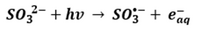
| + | Among the electron source chemicals, sulfite (SO<sub>3</sub><sup>2−</sup>) has emerged as one of the most effective and practical options for generating hydrated electrons to destroy PFAS in water. The mechanism of hydrated electron production in a sulfite solution under ultraviolet is shown in Equation 1 (UV is denoted as ''hv, SO<sub>3</sub><sup><big>'''•-'''</big></sup>'' is the sulfur trioxide radical anion): |
| | + | </br> |
| | + | ::<big>'''Equation 1:'''</big> [[File: XiongEq1.png | 200 px]] |
| | | | |
| − | Knowing the identity of and reaction order in the reductant is required to derive the second-order rate constants listed in Table 1. This same reason limits the utility of reduction rate constants measured with complex carbonaceous reductants such as NOM<ref name="Dunnivant1992"/>, BC<ref name="Oh2013"/><ref name="Oh2009"/><ref name="Xu2015"/><ref name="Xin2021">Xin, D., 2021. Understanding the Electron Storage Capacity of Pyrogenic Black Carbon: Origin, Redox Reversibility, Spatial Distribution, and Environmental Applications. Doctoral Thesis, University of Delaware. [https://udspace.udel.edu/bitstream/handle/19716/30105/Xin_udel_0060D_14728.pdf?sequence=1 Free download.]</ref>, and HS<ref name="Luan2010"/><ref name="Murillo-Gelvez2021"/>, whose chemical structures and redox moieties responsible for the reduction, as well as their abundance, are not clearly defined or known. In other words, the observed rate constants in those studies are specific to the experimental conditions (e.g., pH and NOM source and concentration), and may not be easily comparable to other studies.
| + | The hydrated electron has demonstrated excellent performance in destroying PFAS such as [[Wikipedia:Perfluorooctanesulfonic acid | perfluorooctanesulfonic acid (PFOS)]], [[Wikipedia:Perfluorooctanoic acid|perfluorooctanoic acid (PFOA)]]<ref>Gu, Y., Liu, T., Wang, H., Han, H., Dong, W., 2017. Hydrated Electron Based Decomposition of Perfluorooctane Sulfonate (PFOS) in the VUV/Sulfite System. Science of The Total Environment, 607-608, pp. 541-48. [https://doi.org/10.1016/j.scitotenv.2017.06.197 doi: 10.1016/j.scitotenv.2017.06.197]</ref> and [[Wikipedia: GenX|GenX]]<ref>Bao, Y., Deng, S., Jiang, X., Qu, Y., He, Y., Liu, L., Chai, Q., Mumtaz, M., Huang, J., Cagnetta, G., Yu, G., 2018. Degradation of PFOA Substitute: GenX (HFPO–DA Ammonium Salt): Oxidation with UV/Persulfate or Reduction with UV/Sulfite? Environmental Science and Technology, 52(20), pp. 11728-34. [https://doi.org/10.1021/acs.est.8b02172 doi: 10.1021/acs.est.8b02172]</ref>. Mechanisms include cleaving carbon-to-fluorine (C-F) bonds (i.e., hydrogen/fluorine atom exchange) and chain shortening (i.e., [[Wikipedia: Decarboxylation | decarboxylation]], [[Wikipedia: Hydroxylation | hydroxylation]], [[Wikipedia: Elimination reaction | elimination]], and [[Wikipedia: Hydrolysis | hydrolysis]])<ref name="BentelEtAl2019"/>. |
| | | | |
| − | {| class="wikitable mw-collapsible" style="float:left; margin-right:40px; text-align:center;"
| + | ==Process Description== |
| − | |+ Table 1. Aqueous phase one electron reduction potentials and logarithm of second-order rate constants for the reduction of NACs and MCs by the singly deprotonated form of the hydroquinones lawsone, juglone, AHQDS and AHQS, with the second-order rate constants for the deprotonated NAC/MC species (i.e., nitrophenolates and NTO<sup>–</sup>) in parentheses.
| + | A commercial UV/sulfite treatment system designed and developed by Haley and Aldrich (EradiFluor<sup><small>TM</small></sup><ref name="EradiFluor"/>) includes an optional pre-oxidation step to transform PFAS precursors (when present) and a main treatment step to break C-F bonds by UV/sulfite reduction. The effluent from the treatment process can be sent back to the influent of a pre-treatment separation system (such as a [[Wikipedia: Foam fractionation | foam fractionation]], [[PFAS Treatment by Anion Exchange | regenerable ion exchange]], or a [[Reverse Osmosis and Nanofiltration Membrane Filtration Systems for PFAS Removal | membrane filtration system]]) for further concentration or sent for off-site disposal in accordance with relevant disposal regulations. A conceptual treatment process diagram is shown in Figure 1. [[File: XiongFig1.png | thumb | left | 600 px | Figure 1: Conceptual Treatment Process for a Concentrated PFAS Stream]]<br clear="left"/> |
| − | |-
| |
| − | ! Compound
| |
| − | ! rowspan="2" |''E<sub>H</sub><sup>1'</sup>'' (V)
| |
| − | ! colspan="4"| Hydroquinone [log ''k<sub>R</sub>'' (M<sup>-1</sup>s<sup>-1</sup>)]
| |
| − | |-
| |
| − | ! (NAC/MC)
| |
| − | ! LAW<sup>-</sup>
| |
| − | ! JUG<sup>-</sup>
| |
| − | ! AHQDS<sup>-</sup>
| |
| − | ! AHQS<sup>-</sup>
| |
| − | |-
| |
| − | | Nitrobenzene (NB) || -0.485<ref name="Schwarzenbach1990"/> || 0.380<ref name="Schwarzenbach1990"/> || -1.102<ref name="Schwarzenbach1990"/> || 2.050<ref name="Murillo-Gelvez2019"/> || 3.060<ref name="Murillo-Gelvez2019"/>
| |
| − | |-
| |
| − | | 2-nitrotoluene (2-NT) || -0.590<ref name="Schwarzenbach1990"/> || -1.432<ref name="Schwarzenbach1990"/> || -2.523<ref name="Schwarzenbach1990"/> || 0.775<ref name="Hartenbach2008"/> ||
| |
| − | |-
| |
| − | | 3-nitrotoluene (3-NT) || -0.475<ref name="Schwarzenbach1990"/> || 0.462<ref name="Schwarzenbach1990"/> || -0.921<ref name="Schwarzenbach1990"/> || ||
| |
| − | |-
| |
| − | | 4-nitrotoluene (4-NT) || -0.500<ref name="Schwarzenbach1990"/> || 0.041<ref name="Schwarzenbach1990"/> || -1.292<ref name="Schwarzenbach1990"/> || 1.822<ref name="Hartenbach2008"/> || 2.610<ref name="Murillo-Gelvez2019"/>
| |
| − | |-
| |
| − | | 2-chloronitrobenzene (2-ClNB) || -0.485<ref name="Schwarzenbach1990"/> || 0.342<ref name="Schwarzenbach1990"/> || -0.824<ref name="Schwarzenbach1990"/> ||2.412<ref name="Hartenbach2008"/> ||
| |
| − | |-
| |
| − | | 3-chloronitrobenzene (3-ClNB) || -0.405<ref name="Schwarzenbach1990"/> || 1.491<ref name="Schwarzenbach1990"/> || 0.114<ref name="Schwarzenbach1990"/> || ||
| |
| − | |-
| |
| − | | 4-chloronitrobenzene (4-ClNB) || -0.450<ref name="Schwarzenbach1990"/> || 1.041<ref name="Schwarzenbach1990"/> || -0.301<ref name="Schwarzenbach1990"/> || 2.988<ref name="Hartenbach2008"/> ||
| |
| − | |-
| |
| − | | 2-acetylnitrobenzene (2-AcNB) || -0.470<ref name="Schwarzenbach1990"/> || 0.519<ref name="Schwarzenbach1990"/> || -0.456<ref name="Schwarzenbach1990"/> || ||
| |
| − | |-
| |
| − | | 3-acetylnitrobenzene (3-AcNB) || -0.405<ref name="Schwarzenbach1990"/> || 1.663<ref name="Schwarzenbach1990"/> || 0.398<ref name="Schwarzenbach1990"/> || ||
| |
| − | |-
| |
| − | | 4-acetylnitrobenzene (4-AcNB) || -0.360<ref name="Schwarzenbach1990"/> || 2.519<ref name="Schwarzenbach1990"/> || 1.477<ref name="Schwarzenbach1990"/> || ||
| |
| − | |-
| |
| − | | 2-nitrophenol (2-NP) || || 0.568 (0.079)<ref name="Schwarzenbach1990"/> || || ||
| |
| − | |-
| |
| − | | 4-nitrophenol (4-NP) || || -0.699 (-1.301)<ref name="Schwarzenbach1990"/> || || ||
| |
| − | |-
| |
| − | | 4-methyl-2-nitrophenol (4-Me-2-NP) || || 0.748 (0.176)<ref name="Schwarzenbach1990"/> || || ||
| |
| − | |-
| |
| − | | 4-chloro-2-nitrophenol (4-Cl-2-NP) || || 1.602 (1.114)<ref name="Schwarzenbach1990"/> || || ||
| |
| − | |-
| |
| − | | 5-fluoro-2-nitrophenol (5-Cl-2-NP) || || 0.447 (-0.155)<ref name="Schwarzenbach1990"/> || || ||
| |
| − | |-
| |
| − | | 2,4,6-trinitrotoluene (TNT) || -0.280<ref name="Schwarzenbach2016"/> || || 2.869<ref name="Hofstetter1999"/> || 5.204<ref name="Hartenbach2008"/> ||
| |
| − | |-
| |
| − | | 2-amino-4,6-dinitrotoluene (2-A-4,6-DNT) || -0.400<ref name="Schwarzenbach2016"/> || || 0.987<ref name="Hofstetter1999"/> || ||
| |
| − | |-
| |
| − | | 4-amino-2,6-dinitrotoluene (4-A-2,6-DNT) || -0.440<ref name="Schwarzenbach2016"/> || || 0.079<ref name="Hofstetter1999"/> || ||
| |
| − | |-
| |
| − | | 2,4-diamino-6-nitrotoluene (2,4-DA-6-NT) || -0.505<ref name="Schwarzenbach2016"/> || || -1.678<ref name="Hofstetter1999"/> || ||
| |
| − | |-
| |
| − | | 2,6-diamino-4-nitrotoluene (2,6-DA-4-NT) || -0.495<ref name="Schwarzenbach2016"/> || || -1.252<ref name="Hofstetter1999"/> || ||
| |
| − | |-
| |
| − | | 1,3-dinitrobenzene (1,3-DNB) || -0.345<ref name="Hofstetter1999"/> || || 1.785<ref name="Hofstetter1999"/> || ||
| |
| − | |-
| |
| − | | 1,4-dinitrobenzene (1,4-DNB) || -0.257<ref name="Hofstetter1999"/> || || 3.839<ref name="Hofstetter1999"/> || ||
| |
| − | |-
| |
| − | | 2-nitroaniline (2-NANE) || < -0.560<ref name="Hofstetter1999"/> || || -2.638<ref name="Hofstetter1999"/> || ||
| |
| − | |-
| |
| − | | 3-nitroaniline (3-NANE) || -0.500<ref name="Hofstetter1999"/> || || -1.367<ref name="Hofstetter1999"/> || ||
| |
| − | |-
| |
| − | | 1,2-dinitrobenzene (1,2-DNB) || -0.290<ref name="Hofstetter1999"/> || || || 5.407<ref name="Hartenbach2008"/> ||
| |
| − | |-
| |
| − | | 4-nitroanisole (4-NAN) || || -0.661<ref name="Murillo-Gelvez2019"/> || || 1.220<ref name="Murillo-Gelvez2019"/> ||
| |
| − | |-
| |
| − | | 2-amino-4-nitroanisole (2-A-4-NAN) || || -0.924<ref name="Murillo-Gelvez2019"/> || || 1.150<ref name="Murillo-Gelvez2019"/> || 2.190<ref name="Murillo-Gelvez2019"/>
| |
| − | |-
| |
| − | | 4-amino-2-nitroanisole (4-A-2-NAN) || || || ||1.610<ref name="Murillo-Gelvez2019"/> || 2.360<ref name="Murillo-Gelvez2019"/>
| |
| − | |-
| |
| − | | 2-chloro-4-nitroaniline (2-Cl-5-NANE) || || -0.863<ref name="Murillo-Gelvez2019"/> || || 1.250<ref name="Murillo-Gelvez2019"/> || 2.210<ref name="Murillo-Gelvez2019"/>
| |
| − | |-
| |
| − | | N-methyl-4-nitroaniline (MNA) || || -1.740<ref name="Murillo-Gelvez2019"/> || || -0.260<ref name="Murillo-Gelvez2019"/> || 0.692<ref name="Murillo-Gelvez2019"/>
| |
| − | |-
| |
| − | | 3-nitro-1,2,4-triazol-5-one (NTO) || || || || 5.701 (1.914)<ref name="Murillo-Gelvez2021"/> ||
| |
| − | |-
| |
| − | | Hexahydro-1,3,5-trinitro-1,3,5-triazine (RDX) || || || || -0.349<ref name="Kwon2008"/> ||
| |
| − | |}
| |
| | | | |
| − | [[File:AbioMCredFig5.png | thumb |500px|Figure 5. Relative reduction rate constants of the NACs/MCs listed in Table 1 for AHQDS<sup>–</sup>. Rate constants are compared with respect to RDX. Abbreviations of NACs/MCs as listed in Table 1.]]
| + | ==Advantages== |
| − | Most of the current knowledge about MC degradation is derived from studies using NACs. The reduction kinetics of only four MCs, namely TNT, N-methyl-4-nitroaniline (MNA), NTO, and RDX, have been investigated with hydroquinones. Of these four MCs, only the reduction rates of MNA and TNT have been modeled<ref name="Hofstetter1999"/><ref name="Murillo-Gelvez2019"/><ref name="Riefler2000">Riefler, R.G., and Smets, B.F., 2000. Enzymatic Reduction of 2,4,6-Trinitrotoluene and Related Nitroarenes: Kinetics Linked to One-Electron Redox Potentials. Environmental Science and Technology, 34(18), pp. 3900–3906. [https://doi.org/10.1021/es991422f DOI: 10.1021/es991422f]</ref><ref name="Salter-Blanc2015">Salter-Blanc, A.J., Bylaska, E.J., Johnston, H.J., and Tratnyek, P.G., 2015. Predicting Reduction Rates of Energetic Nitroaromatic Compounds Using Calculated One-Electron Reduction Potentials. Environmental Science and Technology, 49(6), pp. 3778–3786. [https://doi.org/10.1021/es505092s DOI: 10.1021/es505092s] [https://pubs.acs.org/doi/pdf/10.1021/es505092s Open access article.]</ref>.
| + | A UV/sulfite treatment system offers significant advantages for PFAS destruction compared to other technologies, including high defluorination percentage, high treatment efficiency for short-chain PFAS without mass transfer limitation, selective reactivity by ''e<sub><small>aq</small></sub><sup><big>'''-'''</big></sup>'', low energy consumption, and the production of no harmful byproducts. A summary of these advantages is provided below: |
| | + | *'''High efficiency for short- and ultrashort-chain PFAS:''' While the degradation efficiency for short-chain PFAS is challenging for some treatment technologies<ref>Singh, R.K., Brown, E., Mededovic Thagard, S., Holson, T.M., 2021. Treatment of PFAS-containing landfill leachate using an enhanced contact plasma reactor. Journal of Hazardous Materials, 408, Article 124452. [https://doi.org/10.1016/j.jhazmat.2020.124452 doi: 10.1016/j.jhazmat.2020.124452]</ref><ref>Singh, R.K., Multari, N., Nau-Hix, C., Woodard, S., Nickelsen, M., Mededovic Thagard, S., Holson, T.M., 2020. Removal of Poly- and Per-Fluorinated Compounds from Ion Exchange Regenerant Still Bottom Samples in a Plasma Reactor. Environmental Science and Technology, 54(21), pp. 13973-80. [https://doi.org/10.1021/acs.est.0c02158 doi: 10.1021/acs.est.0c02158]</ref><ref>Nau-Hix, C., Multari, N., Singh, R.K., Richardson, S., Kulkarni, P., Anderson, R.H., Holsen, T.M., Mededovic Thagard S., 2021. Field Demonstration of a Pilot-Scale Plasma Reactor for the Rapid Removal of Poly- and Perfluoroalkyl Substances in Groundwater. American Chemical Society’s Environmental Science and Technology (ES&T) Water, 1(3), pp. 680-87. [https://doi.org/10.1021/acsestwater.0c00170 doi: 10.1021/acsestwater.0c00170]</ref>, the UV/sulfite process demonstrates excellent defluorination efficiency for both short- and ultrashort-chain PFAS, including [[Wikipedia: Trifluoroacetic acid | trifluoroacetic acid (TFA)]] and [[Wikipedia: Perfluoropropionic acid | perfluoropropionic acid (PFPrA)]]. |
| | + | *'''High defluorination ratio:''' As shown in Figure 3, the UV/sulfite treatment system has demonstrated near 100% defluorination for various PFAS under both laboratory and field conditions. |
| | + | *'''No harmful byproducts:''' While some oxidative technologies, such as electrochemical oxidation, generate toxic byproducts, including perchlorate, bromate, and chlorate, the UV/sulfite system employs a reductive mechanism and does not generate these byproducts. |
| | + | *'''Ambient pressure and low temperature:''' The system operates under ambient pressure and low temperature (<60°C), as it utilizes UV light and common chemicals to degrade PFAS. |
| | + | *'''Low energy consumption:''' The electrical energy per order values for the degradation of [[Wikipedia: Perfluoroalkyl carboxylic acids | perfluorocarboxylic acids (PFCAs)]] by UV/sulfite have been reduced to less than 1.5 kilowatt-hours (kWh) per cubic meter under laboratory conditions. The energy consumption is orders of magnitude lower than that for many other destructive PFAS treatment technologies (e.g., [[Supercritical Water Oxidation (SCWO) | supercritical water oxidation]])<ref>Nzeribe, B.N., Crimi, M., Mededovic Thagard, S., Holsen, T.M., 2019. Physico-Chemical Processes for the Treatment of Per- And Polyfluoroalkyl Substances (PFAS): A Review. Critical Reviews in Environmental Science and Technology, 49(10), pp. 866-915. [https://doi.org/10.1080/10643389.2018.1542916 doi: 10.1080/10643389.2018.1542916]</ref>. |
| | + | *'''Co-contaminant destruction:''' The UV/sulfite system has also been reported effective in destroying certain co-contaminants in wastewater. For example, UV/sulfite is reported to be effective in reductive dechlorination of chlorinated volatile organic compounds, such as trichloroethene, 1,2-dichloroethane, and vinyl chloride<ref>Jung, B., Farzaneh, H., Khodary, A., Abdel-Wahab, A., 2015. Photochemical degradation of trichloroethylene by sulfite-mediated UV irradiation. Journal of Environmental Chemical Engineering, 3(3), pp. 2194-2202. [https://doi.org/10.1016/j.jece.2015.07.026 doi: 10.1016/j.jece.2015.07.026]</ref><ref>Liu, X., Yoon, S., Batchelor, B., Abdel-Wahab, A., 2013. Photochemical degradation of vinyl chloride with an Advanced Reduction Process (ARP) – Effects of reagents and pH. Chemical Engineering Journal, 215-216, pp. 868-875. [https://doi.org/10.1016/j.cej.2012.11.086 doi: 10.1016/j.cej.2012.11.086]</ref><ref>Li, X., Ma, J., Liu, G., Fang, J., Yue, S., Guan, Y., Chen, L., Liu, X., 2012. Efficient Reductive Dechlorination of Monochloroacetic Acid by Sulfite/UV Process. Environmental Science and Technology, 46(13), pp. 7342-49. [https://doi.org/10.1021/es3008535 doi: 10.1021/es3008535]</ref><ref>Li, X., Fang, J., Liu, G., Zhang, S., Pan, B., Ma, J., 2014. Kinetics and efficiency of the hydrated electron-induced dehalogenation by the sulfite/UV process. Water Research, 62, pp. 220-228. [https://doi.org/10.1016/j.watres.2014.05.051 doi: 10.1016/j.watres.2014.05.051]</ref>. |
| | | | |
| − | Using the rate constants obtained with AHQDS<sup>–</sup>, a relative reactivity trend can be obtained (Figure 5). RDX is the slowest reacting MC in Table 1, hence it was selected to calculate the relative rates of reaction (i.e., log ''k<sub>NAC/MC</sub>'' – log ''k<sub>RDX</sub>''). If only the MCs in Figure 5 are considered, the reactivity spans 6 orders of magnitude following the trend: RDX ≈ MNA < NTO<sup>–</sup> < DNAN < TNT < NTO. The rate constant for DNAN reduction by AHQDS<sup>–</sup> is not yet published and hence not included in Table 1. Note that speciation of NACs/MCs can significantly affect their reduction rates. Upon deprotonation, the NAC/MC becomes negatively charged and less reactive as an oxidant (i.e., less prone to accept an electron). As a result, the second-order rate constant can decrease by 0.5-0.6 log unit in the case of nitrophenols and approximately 4 log units in the case of NTO (numbers in parentheses in Table 1)<ref name="Schwarzenbach1990"/><ref name="Murillo-Gelvez2021"/>.
| + | ==Limitations== |
| | + | Several environmental factors and potential issues have been identified that may impact the performance of the UV/sulfite treatment system, as listed below. Solutions to address these issues are also proposed. |
| | + | *Environmental factors, such as the presence of elevated concentrations of natural organic matter (NOM), dissolved oxygen, or nitrate, can inhibit the efficacy of UV/sulfite treatment systems by scavenging available hydrated electrons. Those interferences are commonly managed through chemical additions, reaction optimization, and/or dilution, and are therefore not considered likely to hinder treatment success. |
| | + | *Coloration in waste streams may also impact the effectiveness of the UV/sulfite treatment system by blocking the transmission of UV light, thus reducing the UV lamp's effective path length. To address this, pre-treatment may be necessary to enable UV/sulfite destruction of PFAS in the waste stream. Pre-treatment may include the use of strong oxidants or coagulants to consume or remove UV-absorbing constituents. |
| | + | *The degradation efficiency is strongly influenced by PFAS molecular structure, with fluorotelomer sulfonates (FTS) and [[Wikipedia: Perfluorobutanesulfonic acid | perfluorobutanesulfonate (PFBS)]] exhibiting greater resistance to degradation by UV/sulfite treatment compared to other PFAS compounds. |
| | | | |
| − | ==Ferruginous Reductants== | + | ==State of the Practice== |
| − | {| class="wikitable mw-collapsible" style="float:right; margin-left:40px; text-align:center;"
| + | [[File: XiongFig2.png | thumb | 500 px | Figure 2. Field demonstration of EradiFluor<sup><small>TM</small></sup><ref name="EradiFluor"/> for PFAS destruction in a concentrated waste stream in a Mid-Atlantic Naval Air Station: a) Target PFAS at each step of the treatment shows that about 99% of PFAS were destroyed; meanwhile, the final degradation product, i.e., fluoride, increased to 15 mg/L in concentration, demonstrating effective PFAS destruction; b) AOF concentrations at each step of the treatment provided additional evidence to show near-complete mineralization of PFAS. Average results from multiple batches of treatment are shown here.]] |
| − | |+ Table 2. Logarithm of second-order rate constants for reduction of NACs and MCs by dissolved Fe(II) complexes with the stoichiometry of ligand and iron in square brackets
| + | [[File: XiongFig3.png | thumb | 500 px | Figure 3. Field demonstration of a treatment train (SAFF + EradiFluor<sup><small>TM</small></sup><ref name="EradiFluor"/>) for groundwater PFAS separation and destruction at an Air Force base in California: a) Two main components of the treatment train, i.e. SAFF and EradiFluor<sup><small>TM</small></sup><ref name="EradiFluor"/>; b) Results showed the effective destruction of various PFAS in the foam fractionate. The target PFAS at each step of the treatment shows that about 99.9% of PFAS were destroyed. Meanwhile, the final degradation product, i.e., fluoride, increased to 30 mg/L in concentration, demonstrating effective destruction of PFAS in a foam fractionate concentrate. After a polishing treatment step (GAC) via the onsite groundwater extraction and treatment system, all PFAS were removed to concentrations below their MCLs.]] |
| − | |- | + | The effectiveness of UV/sulfite technology for treating PFAS has been evaluated in two field demonstrations using the EradiFluor<sup><small>TM</small></sup><ref name="EradiFluor"/> system. Aqueous samples collected from the system were analyzed using EPA Method 1633, the [[Wikipedia: TOP Assay | total oxidizable precursor (TOP) assay]], adsorbable organic fluorine (AOF) method, and non-target analysis. A summary of each demonstration and their corresponding PFAS treatment efficiency is provided below. |
| − | ! rowspan="2" | Compound
| + | *Under the [https://serdp-estcp.mil/ Environmental Security Technology Certification Program (ESTCP)] [https://serdp-estcp.mil/projects/details/4c073623-e73e-4f07-a36d-e35c7acc75b6/er21-5152-project-overview Project ER21-5152], a field demonstration of EradiFluor<sup><small>TM</small></sup><ref name="EradiFluor"/> was conducted at a Navy site on the east coast, and results showed that the technology was highly effective in destroying various PFAS in a liquid concentrate produced from an ''in situ'' foam fractionation groundwater treatment system. As shown in Figure 2a, total PFAS concentrations were reduced from 17,366 micrograms per liter (µg/L) to 195 µg/L at the end of the UV/sulfite reaction, representing 99% destruction. After the ion exchange resin polishing step, all residual PFAS had been removed to the non-detect level, except one compound (PFOS) reported as 1.5 nanograms per liter (ng/L), which is below the current Maximum Contaminant Level (MCL) of 4 ng/L. Meanwhile, the fluoride concentration increased up to 15 milligrams per liter (mg/L), confirming near complete defluorination. Figure 2b shows the adsorbable organic fluorine results from the same treatment test, which similarly demonstrates destruction of 99% of PFAS. |
| − | ! rowspan="2" | E<sub>H</sub><sup>1'</sup> (V)
| + | *Another field demonstration was completed at an Air Force base in California, where a treatment train combining [https://serdp-estcp.mil/projects/details/263f9b50-8665-4ecc-81bd-d96b74445ca2 Surface Active Foam Fractionation (SAFF)] and EradiFluor<sup><small>TM</small></sup><ref name="EradiFluor"/> was used to treat PFAS in groundwater. As shown in Figure 3, PFAS analytical data and fluoride results demonstrated near-complete destruction of various PFAS. In addition, this demonstration showed: a) high PFAS destruction ratio was achieved in the foam fractionate, even in very high concentration (up to 1,700 mg/L of booster), and b) the effluent from EradiFluor<sup><small>TM</small></sup><ref name="EradiFluor"/> was sent back to the influent of the SAFF system for further concentration and treatment, resulting in a closed-loop treatment system and no waste discharge from EradiFluor<sup><small>TM</small></sup><ref name="EradiFluor"/>. This field demonstration was conducted with the approval of three regulatory agencies (United States Environmental Protection Agency, California Regional Water Quality Control Board, and California Department of Toxic Substances Control). |
| − | ! Cysteine<ref name="Naka2008"/></br>[FeL<sub>2</sub>]<sup>2-</sup>
| |
| − | ! Thioglycolic acid<ref name="Naka2008"/></br>[FeL<sub>2</sub>]<sup>2-</sup>
| |
| − | ! DFOB<ref name="Kim2009"/></br>[FeHL]<sup>0</sup>
| |
| − | ! AcHA<ref name="Kim2009"/></br>[FeL<sub>3</sub>]<sup>-</sup>
| |
| − | ! Tiron <sup>a</sup></br>[FeL<sub>2</sub>]<sup>6-</sup>
| |
| − | ! Fe-Porphyrin <sup>b</sup>
| |
| − | |-
| |
| − | ! colspan="6" | Fe(II)-Ligand [log ''k<sub>R</sub>'' (M<sup>-1</sup>s<sup>-1</sup>)]
| |
| − | |-
| |
| − | | Nitrobenzene || -0.485<ref name="Schwarzenbach1990"/> || -0.347 || 0.874 || 2.235 || -0.136 || 1.424<ref name="Gao2021">Gao, Y., Zhong, S., Torralba-Sanchez, T.L., Tratnyek, P.G., Weber, E.J., Chen, Y., and Zhang, H., 2021. Quantitative structure activity relationships (QSARs) and machine learning models for abiotic reduction of organic compounds by an aqueous Fe(II) complex. Water Research, 192, p. 116843. [https://doi.org/10.1016/j.watres.2021.116843 DOI: 10.1016/j.watres.2021.116843]</ref></br>4.000<ref name="Salter-Blanc2015"/> || -0.018<ref name="Schwarzenbach1990"/></br>0.026<ref name="Salter-Blanc2015"/>
| |
| − | |-
| |
| − | | 2-nitrotoluene || -0.590<ref name="Schwarzenbach1990"/> || || || || || || -0.602<ref name="Schwarzenbach1990"/>
| |
| − | |-
| |
| − | | 3-nitrotoluene || -0.475<ref name="Schwarzenbach1990"/> || -0.434 || 0.767 || 2.106 || -0.229 || 1.999<ref name="Gao2021"/></br>3.800<ref name="Salter-Blanc2015"/> || 0.041<ref name="Schwarzenbach1990"/>
| |
| − | |-
| |
| − | | 4-nitrotoluene || -0.500<ref name="Schwarzenbach1990"/> || -0.652 || 0.528 || 2.013 || -0.402 || 1.446<ref name="Gao2021"/></br>3.500<ref name="Salter-Blanc2015"/> || -0.174<ref name="Schwarzenbach1990"/>
| |
| − | |-
| |
| − | | 2-chloronitrobenzene || -0.485<ref name="Schwarzenbach1990"/> || || || || || || 0.944<ref name="Schwarzenbach1990"/>
| |
| − | |-
| |
| − | | 3-chloronitrobenzene || -0.405<ref name="Schwarzenbach1990"/> || 0.360 || 1.810 || 2.888 || 0.691 || 2.882<ref name="Gao2021"/></br>4.900<ref name="Salter-Blanc2015"/> || 0.724<ref name="Schwarzenbach1990"/>
| |
| − | |-
| |
| − | | 4-chloronitrobenzene || -0.450<ref name="Schwarzenbach1990"/> || 0.230 || 1.415 || 2.512 || 0.375 || 3.937<ref name="Gao2021"/></br>4.581<ref name="Naka2006"/> || 0.431<ref name="Schwarzenbach1990"/></br>0.289<ref name="Salter-Blanc2015"/>
| |
| − | |-
| |
| − | | 2-acetylnitrobenzene || -0.470<ref name="Schwarzenbach1990"/> || || || || || || 1.377<ref name="Schwarzenbach1990"/>
| |
| − | |-
| |
| − | | 3-acetylnitrobenzene || -0.405<ref name="Schwarzenbach1990"/> || || || || || || 0.799<ref name="Schwarzenbach1990"/>
| |
| − | |-
| |
| − | | 4-acetylnitrobenzene || -0.360<ref name="Schwarzenbach1990"/> || 0.965 || 2.771 || || 1.872 || 5.028<ref name="Gao2021"/></br>6.300<ref name="Salter-Blanc2015"/> || 1.693<ref name="Schwarzenbach1990"/>
| |
| − | |-
| |
| − | | RDX || -0.550<ref name="Uchimiya2010">Uchimiya, M., Gorb, L., Isayev, O., Qasim, M.M., and Leszczynski, J., 2010. One-electron standard reduction potentials of nitroaromatic and cyclic nitramine explosives. Environmental Pollution, 158(10), pp. 3048–3053. [https://doi.org/10.1016/j.envpol.2010.06.033 DOI: 10.1016/j.envpol.2010.06.033]</ref> || || || || || 2.212<ref name="Gao2021"/></br>2.864<ref name="Kim2007"/> ||
| |
| − | |-
| |
| − | | HMX || -0.660<ref name="Uchimiya2010"/> || || || || || -2.762<ref name="Gao2021"/> ||
| |
| − | |-
| |
| − | | TNT || -0.280<ref name="Schwarzenbach2016"/> || || || || || 7.427<ref name="Gao2021"/> || 2.050<ref name="Salter-Blanc2015"/>
| |
| − | |-
| |
| − | | 1,3-dinitrobenzene || -0.345<ref name="Hofstetter1999"/> || || || || || || 1.220<ref name="Salter-Blanc2015"/>
| |
| − | |-
| |
| − | | 2,4-dinitrotoluene || -0.380<ref name="Schwarzenbach2016"/> || || || || || 5.319<ref name="Gao2021"/> || 1.156<ref name="Salter-Blanc2015"/>
| |
| − | |-
| |
| − | | Nitroguanidine (NQ) || -0.700<ref name="Uchimiya2010"/> || || || || || -0.185<ref name="Gao2021"/> ||
| |
| − | |-
| |
| − | | 2,4-dinitroanisole (DNAN) || -0.400<ref name="Uchimiya2010"/> || || || || || || 1.243<ref name="Salter-Blanc2015"/>
| |
| − | |-
| |
| − | | colspan="8" style="text-align:left; background-color:white;" | Notes:</br>''<sup>a</sup>'' 4,5-dihydroxybenzene-1,3-disulfonate (Tiron). ''<sup>b</sup>'' meso-tetra(N-methyl-pyridyl)iron porphin in cysteine.
| |
| − | |}
| |
| − | {| class="wikitable mw-collapsible" style="float:left; margin-right:40px; text-align:center;"
| |
| − | |+ Table 3. Rate constants for the reduction of MCs by iron minerals
| |
| − | |-
| |
| − | ! MC
| |
| − | ! Iron Mineral
| |
| − | ! Iron mineral loading</br>(g/L)
| |
| − | ! Surface area</br>(m<sup>2</sup>/g)
| |
| − | ! Fe(II)<sub>aq</sub> initial</br>(mM) ''<sup>b</sup>''
| |
| − | ! Fe(II)<sub>aq</sub> after 24 h</br>(mM) ''<sup>c</sup>''
| |
| − | ! Fe(II)<sub>aq</sub> sorbed</br>(mM) ''<sup>d</sup>''
| |
| − | ! pH
| |
| − | ! Buffer
| |
| − | ! Buffer</br>(mM)
| |
| − | ! MC initial</br>(μM) ''<sup>e</sup>''
| |
| − | ! log ''k<sub>obs</sub>''</br>(h<sup>-1</sup>) ''<sup>f</sup>''
| |
| − | ! log ''k<sub>SA</sub>''</br>(Lh<sup>-1</sup>m<sup>-2</sup>) ''<sup>g</sup>''
| |
| − | |-
| |
| − | | TNT<ref name="Hofstetter1999"/> || Goethite || 0.64 || 17.5 || 1.5 || || || 7.0 || MOPS || 25 || 50 || 1.200 || 0.170
| |
| − | |-
| |
| − | | RDX<ref name="Gregory2004"/> || Magnetite || 1.00 || 44 || 0.1 || 0 || 0.10 || 7.0 || HEPES || 50 || 50 || -3.500 || -5.200
| |
| − | |-
| |
| − | | RDX<ref name="Gregory2004"/> || Magnetite || 1.00 || 44 || 0.2 || 0.02 || 0.18 || 7.0 || HEPES || 50 || 50 || -2.900 || -4.500
| |
| − | |-
| |
| − | | RDX<ref name="Gregory2004"/> || Magnetite || 1.00 || 44 || 0.5 || 0.23 || 0.27 || 7.0 || HEPES || 50 || 50 || -1.900 || -3.600
| |
| − | |-
| |
| − | | RDX<ref name="Gregory2004"/> || Magnetite || 1.00 || 44 || 1.5 || 0.94 || 0.56 || 7.0 || HEPES || 50 || 50 || -1.400 || -3.100
| |
| − | |-
| |
| − | | RDX<ref name="Gregory2004"/> || Magnetite || 1.00 || 44 || 3.0 || 1.74 || 1.26 || 7.0 || HEPES || 50 || 50 || -1.200 || -2.900
| |
| − | |-
| |
| − | | RDX<ref name="Gregory2004"/> || Magnetite || 1.00 || 44 || 5.0 || 3.38 || 1.62 || 7.0 || HEPES || 50 || 50 || -1.100 || -2.800
| |
| − | |-
| |
| − | | RDX<ref name="Gregory2004"/> || Magnetite || 1.00 || 44 || 10.0 || 7.77 || 2.23 || 7.0 || HEPES || 50 || 50 || -1.000 || -2.600
| |
| − | |-
| |
| − | | RDX<ref name="Gregory2004"/> || Magnetite || 1.00 || 44 || 1.6 || 1.42 || 0.16 || 6.0 || MES || 50 || 50 || -2.700 || -4.300
| |
| − | |-
| |
| − | | RDX<ref name="Gregory2004"/> || Magnetite || 1.00 || 44 || 1.6 || 1.34 || 0.24 || 6.5 || MOPS || 50 || 50 || -1.800 || -3.400
| |
| − | |-
| |
| − | | RDX<ref name="Gregory2004"/> || Magnetite || 1.00 || 44 || 1.6 || 1.21 || 0.37 || 7.0 || MOPS || 50 || 50 || -1.200 || -2.900
| |
| − | |-
| |
| − | | RDX<ref name="Gregory2004"/> || Magnetite || 1.00 || 44 || 1.6 || 1.01 || 0.57 || 7.0 || HEPES || 50 || 50 || -1.200 || -2.800
| |
| − | |-
| |
| − | | RDX<ref name="Gregory2004"/> || Magnetite || 1.00 || 44 || 1.6 || 0.76 || 0.82 || 7.5 || HEPES || 50 || 50 || -0.490 || -2.100
| |
| − | |-
| |
| − | | RDX<ref name="Gregory2004"/> || Magnetite || 1.00 || 44 || 1.6 || 0.56 || 1.01 || 8.0 || HEPES || 50 || 50 || -0.590 || -2.200
| |
| − | |-
| |
| − | | NG<ref name="Oh2004"/> || Magnetite || 4.00 || 0.56|| 4.0 || || || 7.4 || HEPES || 90 || 226 || ||
| |
| − | |-
| |
| − | | NG<ref name="Oh2008"/> || Pyrite || 20.00 || 0.53 || || || || 7.4 || HEPES || 100 || 307 || -2.213 || -3.238
| |
| − | |-
| |
| − | | TNT<ref name="Oh2008"/> || Pyrite || 20.00 || 0.53 || || || || 7.4 || HEPES || 100 || 242 || -2.812 || -3.837
| |
| − | |-
| |
| − | | RDX<ref name="Oh2008"/> || Pyrite || 20.00 || 0.53 || || || || 7.4 || HEPES || 100 || 201 || -3.058 || -4.083
| |
| − | |-
| |
| − | | RDX<ref name="Larese-Casanova2008"/> || Carbonate Green Rust || 5.00 || 36 || || || || 7.0 || || || 100 || ||
| |
| − | |-
| |
| − | | RDX<ref name="Larese-Casanova2008"/> || Sulfate Green Rust || 5.00 || 20 || || || || 7.0 || || || 100 || ||
| |
| − | |-
| |
| − | | DNAN<ref name="Khatiwada2018"/> || Sulfate Green Rust || 10.00 || || || || || 8.4 || || || 500 || ||
| |
| − | |-
| |
| − | | NTO<ref name="Khatiwada2018"/> || Sulfate Green Rust || 10.00 || || || || || 8.4 || || || 500 || ||
| |
| − | |-
| |
| − | | DNAN<ref name="Berens2019"/> || Magnetite || 2.00 || 17.8 || 1.0 || || || 7.0 || NaHCO<sub>3</sub> || 10 || 200 || -0.100 || -1.700
| |
| − | |-
| |
| − | | DNAN<ref name="Berens2019"/> || Mackinawite || 1.50 || || || || || 7.0 || NaHCO<sub>3</sub> || 10 || 200 || 0.061 ||
| |
| − | |-
| |
| − | | DNAN<ref name="Berens2019"/> || Goethite || 1.00 || 103.8 || 1.0 || || || 7.0 || NaHCO<sub>3</sub> || 10 || 200 || 0.410 || -1.600
| |
| − | |-
| |
| − | | RDX<ref name="Strehlau2018"/> || Magnetite || 0.62 || || 1.0 || || || 7.0 || NaHCO<sub>3</sub> || 10 || 17.5 || -1.100 ||
| |
| − | |-
| |
| − | | RDX<ref name="Strehlau2018"/> || Magnetite || 0.62 || || || || || 7.0 || MOPS || 50 || 17.5 || -0.270 ||
| |
| − | |-
| |
| − | | RDX<ref name="Strehlau2018"/> || Magnetite || 0.62 || || 1.0 || || || 7.0 || MOPS || 10 || 17.6 || -0.480 ||
| |
| − | |-
| |
| − | | NTO<ref name="Cardenas-Hernandez2020"/> || Hematite || 1.00 || 5.7 || 1.0 || 0.92 || 0.08 || 5.5 || MES || 50 || 30 || -0.550 || -1.308
| |
| − | |-
| |
| − | | NTO<ref name="Cardenas-Hernandez2020"/> || Hematite || 1.00 || 5.7 || 1.0 || 0.85 || 0.15 || 6.0 || MES || 50 || 30 || 0.619 || -0.140
| |
| − | |-
| |
| − | | NTO<ref name="Cardenas-Hernandez2020"/> || Hematite || 1.00 || 5.7 || 1.0 || 0.9 || 0.10 || 6.5 || MES || 50 || 30 || 1.348 || 0.590
| |
| − | |-
| |
| − | | NTO<ref name="Cardenas-Hernandez2020"/> || Hematite || 1.00 || 5.7 || 1.0 || 0.77 || 0.23 || 7.0 || MOPS || 50 || 30 || 2.167 || 1.408
| |
| − | |-
| |
| − | | NTO<ref name="Cardenas-Hernandez2020"/> || Hematite ''<sup>a</sup>'' || 1.00 || 5.7 || || 1.01 || || 5.5 || MES || 50 || 30 || -1.444 || -2.200
| |
| − | |-
| |
| − | | NTO<ref name="Cardenas-Hernandez2020"/> || Hematite ''<sup>a</sup>'' || 1.00 || 5.7 || || 0.97 || || 6.0 || MES || 50 || 30 || -0.658 || -1.413
| |
| − | |-
| |
| − | | NTO<ref name="Cardenas-Hernandez2020"/> || Hematite ''<sup>a</sup>'' || 1.00 || 5.7 || || 0.87 || || 6.5 || MES || 50 || 30 || 0.068 || -0.688
| |
| − | |-
| |
| − | | NTO<ref name="Cardenas-Hernandez2020"/> || Hematite ''<sup>a</sup>'' || 1.00 || 5.7 || || 0.79 || || 7.0 || MOPS || 50 || 30 || 1.210 || 0.456
| |
| − | |-
| |
| − | | RDX<ref name="Tong2021"/> || Mackinawite || 0.45 || || || || || 6.5 || NaHCO<sub>3</sub> || 10 || 250 || -0.092 ||
| |
| − | |-
| |
| − | | RDX<ref name="Tong2021"/> || Mackinawite || 0.45 || || || || || 7.0 || NaHCO<sub>3</sub> || 10 || 250 || 0.009 ||
| |
| − | |-
| |
| − | | RDX<ref name="Tong2021"/> || Mackinawite || 0.45 || || || || || 7.5 || NaHCO<sub>3</sub> || 10 || 250 || 0.158 ||
| |
| − | |-
| |
| − | | RDX<ref name="Tong2021"/> || Green Rust || 5 || || || || || 6.5 || NaHCO<sub>3</sub> || 10 || 250 || -1.301 ||
| |
| − | |-
| |
| − | | RDX<ref name="Tong2021"/> || Green Rust || 5 || || || || || 7.0 || NaHCO<sub>3</sub> || 10 || 250 || -1.097 ||
| |
| − | |-
| |
| − | | RDX<ref name="Tong2021"/> || Green Rust || 5 || || || || || 7.5 || NaHCO<sub>3</sub> || 10 || 250 || -0.745 ||
| |
| − | |-
| |
| − | | RDX<ref name="Tong2021"/> || Goethite || 0.5 || || 1 || 1 || || 6.5 || NaHCO<sub>3</sub> || 10 || 250 || -0.921 ||
| |
| − | |-
| |
| − | | RDX<ref name="Tong2021"/> || Goethite || 0.5 || || 1 || 1 || || 7.0 || NaHCO<sub>3</sub> || 10 || 250 || -0.347 ||
| |
| − | |-
| |
| − | | RDX<ref name="Tong2021"/> || Goethite || 0.5 || || 1 || 1 || || 7.5 || NaHCO<sub>3</sub> || 10 || 250 || 0.009 ||
| |
| − | |-
| |
| − | | RDX<ref name="Tong2021"/> || Hematite || 0.5 || || 1 || 1 || || 6.5 || NaHCO<sub>3</sub> || 10 || 250 || -0.824 ||
| |
| − | |-
| |
| − | | RDX<ref name="Tong2021"/> || Hematite || 0.5 || || 1 || 1 || || 7.0 || NaHCO<sub>3</sub> || 10 || 250 || -0.456 ||
| |
| − | |-
| |
| − | | RDX<ref name="Tong2021"/> || Hematite || 0.5 || || 1 || 1 || || 7.5 || NaHCO<sub>3</sub> || 10 || 250 || -0.237 ||
| |
| − | |-
| |
| − | | RDX<ref name="Tong2021"/> || Magnetite || 2 || || 1 || 1 || || 6.5 || NaHCO<sub>3</sub> || 10 || 250 || -1.523 ||
| |
| − | |-
| |
| − | | RDX<ref name="Tong2021"/> || Magnetite || 2 || || 1 || 1 || || 7.0 || NaHCO<sub>3</sub> || 10 || 250 || -0.824 ||
| |
| − | |-
| |
| − | | RDX<ref name="Tong2021"/> || Magnetite || 2 || || 1 || 1 || || 7.5 || NaHCO<sub>3</sub> || 10 || 250 || -0.229 ||
| |
| − | |-
| |
| − | | DNAN<ref name="Menezes2021"/> || Mackinawite || 4.28 || 0.25 || || || || 6.5 || NaHCO<sub>3</sub> || 8.5 + 20% CO<sub>2</sub>(g) || 400 || 0.836 || 0.806
| |
| − | |-
| |
| − | | DNAN<ref name="Menezes2021"/> || Mackinawite || 4.28 || 0.25 || || || || 7.6 || NaHCO<sub>3</sub> || 95.2 + 20% CO<sub>2</sub>(g) || 400 || 0.762 || 0.732
| |
| − | |-
| |
| − | | DNAN<ref name="Menezes2021"/> || Commercial FeS || 5.00 || 0.214 || || || || 6.5 || NaHCO<sub>3</sub> || 8.5 + 20% CO<sub>2</sub>(g) || 400 || 0.477 || 0.447
| |
| − | |-
| |
| − | | DNAN<ref name="Menezes2021"/> || Commercial FeS || 5.00 || 0.214 || || || || 7.6 || NaHCO<sub>3</sub> || 95.2 + 20% CO<sub>2</sub>(g) || 400 || 0.745 || 0.716
| |
| − | |-
| |
| − | | NTO<ref name="Menezes2021"/> || Mackinawite || 4.28 || 0.25 || || || || 6.5 || NaHCO<sub>3</sub> || 8.5 + 20% CO<sub>2</sub>(g) || 1000 || 0.663 || 0.633
| |
| − | |-
| |
| − | | NTO<ref name="Menezes2021"/> || Mackinawite || 4.28 || 0.25 || || || || 7.6 || NaHCO<sub>3</sub> || 95.2 + 20% CO<sub>2</sub>(g) || 1000 || 0.521 || 0.491
| |
| − | |-
| |
| − | | NTO<ref name="Menezes2021"/> || Commercial FeS || 5.00 || 0.214 || || || || 6.5 || NaHCO<sub>3</sub> || 8.5 + 20% CO<sub>2</sub>(g) || 1000 || 0.492 || 0.462
| |
| − | |-
| |
| − | | NTO<ref name="Menezes2021"/> || Commercial FeS || 5.00 || 0.214 || || || || 7.6 || NaHCO<sub>3</sub> || 95.2 + 20% CO<sub>2</sub>(g) || 1000 || 0.427 || 0.398
| |
| − | |-
| |
| − | | colspan="13" style="text-align:left; background-color:white;" | Notes:</br>''<sup>a</sup>'' Dithionite-reduced hematite; experiments conducted in the presence of 1 mM sulfite. ''<sup>b</sup>'' Initial aqueous Fe(II); not added for Fe(II) bearing minerals. ''<sup>c</sup>'' Aqueous Fe(II) after 24h of equilibration. ''<sup>d</sup>'' Difference between b and c. ''<sup>e</sup>'' Initial nominal MC concentration. ''<sup>f</sup>'' Pseudo-first order rate constant. ''<sup>g</sup>'' Surface area normalized rate constant calculated as ''k<sub>Obs</sub>'' '''/''' (surface area concentration) or ''k<sub>Obs</sub>'' '''/''' (surface area × mineral loading).
| |
| − | |}
| |
| − | {| class="wikitable mw-collapsible" style="float:right; margin-left:40px; text-align:center;"
| |
| − | |+ Table 4. Rate constants for the reduction of NACs by iron oxides in the presence of aqueous Fe(II)
| |
| − | |-
| |
| − | ! NAC ''<sup>a</sup>''
| |
| − | ! Iron Oxide
| |
| − | ! Iron oxide loading</br>(g/L)
| |
| − | ! Surface area</br>(m<sup>2</sup>/g)
| |
| − | ! Fe(II)<sub>aq</sub> initial</br>(mM) ''<sup>b</sup>''
| |
| − | ! Fe(II)<sub>aq</sub> after 24 h</br>(mM) ''<sup>c</sup>''
| |
| − | ! Fe(II)<sub>aq</sub> sorbed</br>(mM) ''<sup>d</sup>''
| |
| − | ! pH
| |
| − | ! Buffer
| |
| − | ! Buffer</br>(mM)
| |
| − | ! NAC initial</br>(μM) ''<sup>e</sup>''
| |
| − | ! log ''k<sub>obs</sub>''</br>(h<sup>-1</sup>) ''<sup>f</sup>''
| |
| − | ! log ''k<sub>SA</sub>''</br>(Lh<sup>-1</sup>m<sup>-2</sup>) ''<sup>g</sup>''
| |
| − | |-
| |
| − | | NB<ref name="Klausen1995"/> || Magnetite || 0.200 || 56.00 || 1.5000 || || || 7.00 || Phosphate || 10 || 50 || 1.05E+00 || 7.75E-04
| |
| − | |-
| |
| − | | 4-ClNB<ref name="Klausen1995"/> || Magnetite || 0.200 || 56.00 || 1.5000 || || || 7.00 || Phosphate || 10 || 50 || 1.14E+00 || 8.69E-02
| |
| − | |-
| |
| − | | 4-ClNB<ref name="Hofstetter1999"/> || Goethite || 0.640 || 17.50 || 1.5000 || || || 7.00 || MOPS || 25 || 50 || -1.01E-01 || -1.15E+00
| |
| − | |-
| |
| − | | 4-ClNB<ref name="Elsner2004"/> || Goethite || 1.500 || 16.20 || 1.2400 || 0.9600 || 0.2800 || 7.20 || MOPS || 1.2 || 0.5 - 3 || 1.68E+00 || 2.80E-01
| |
| − | |-
| |
| − | | 4-ClNB<ref name="Elsner2004"/> || Hematite || 1.800 || 13.70 || 1.0400 || 1.0100 || 0.0300 || 7.20 || MOPS || 1.2 || 0.5 - 3 || -2.32E+00 || -3.72E+00
| |
| − | |-
| |
| − | | 4-ClNB<ref name="Elsner2004"/> || Lepidocrocite || 1.400 || 17.60 || 1.1400 || 1.0000 || 0.1400 || 7.20 || MOPS || 1.2 || 0.5 - 3 || 1.51E+00 || 1.20E-01
| |
| − | |-
| |
| − | | 4-CNNB<ref name="Colón2006"/> || Ferrihydrite || 0.004 || 292.00 || 0.3750 || 0.3500 || 0.0300 || 7.97 || HEPES || 25 || 15 || -7.47E-01 || -8.61E-01
| |
| − | |-
| |
| − | | 4-CNNB<ref name="Colón2006"/> || Ferrihydrite || 0.004 || 292.00 || 0.3750 || 0.3700 || 0.0079 || 7.67 || HEPES || 25 || 15 || -1.51E+00 || -1.62E+00
| |
| − | |-
| |
| − | | 4-CNNB<ref name="Colón2006"/> || Ferrihydrite || 0.004 || 292.00 || 0.3750 || 0.3600 || 0.0200 || 7.50 || MOPS || 25 || 15 || -2.15E+00 || -2.26E+00
| |
| − | |-
| |
| − | | 4-CNNB<ref name="Colón2006"/> || Ferrihydrite || 0.004 || 292.00 || 0.3750 || 0.3600 || 0.0120 || 7.28 || MOPS || 25 || 15 || -3.08E+00 || -3.19E+00
| |
| − | |-
| |
| − | | 4-CNNB<ref name="Colón2006"/> || Ferrihydrite || 0.004 || 292.00 || 0.3750 || 0.3700 || 0.0004 || 7.00 || MOPS || 25 || 15 || -3.22E+00 || -3.34E+00
| |
| − | |-
| |
| − | | 4-CNNB<ref name="Colón2006"/> || Ferrihydrite || 0.004 || 292.00 || 0.3750 || 0.3700 || 0.0024 || 6.80 || MOPSO || 25 || 15 || -3.72E+00 || -3.83E+00
| |
| − | |-
| |
| − | | 4-CNNB<ref name="Colón2006"/> || Ferrihydrite || 0.004 || 292.00 || 0.3750 || 0.3700 || 0.0031 || 6.60 || MES || 25 || 15 || -3.83E+00 || -3.94E+00
| |
| − | |-
| |
| − | | 4-CNNB<ref name="Colón2006"/> || Ferrihydrite || 0.020 || 292.00 || 0.3750 || 0.3700 || 0.0031 || 6.60 || MES || 25 || 15 || -3.83E+00 || -4.60E+00
| |
| − | |-
| |
| − | | 4-CNNB<ref name="Colón2006"/> || Ferrihydrite || 0.110 || 292.00 || 0.3750 || 0.3700 || 0.0032 || 6.60 || MES || 25 || 15 || -1.57E+00 || -3.08E+00
| |
| − | |-
| |
| − | | 4-CNNB<ref name="Colón2006"/> || Ferrihydrite || 0.220 || 292.00 || 0.3750 || 0.3700 || 0.0040 || 6.60 || MES || 25 || 15 || -1.12E+00 || -2.93E+00
| |
| − | |-
| |
| − | | 4-CNNB<ref name="Colón2006"/> || Ferrihydrite || 0.551 || 292.00 || 0.3750 || 0.3700 || 0.0092 || 6.60 || MES || 25 || 15 || -6.18E-01 || -2.82E+00
| |
| − | |-
| |
| − | | 4-CNNB<ref name="Colón2006"/> || Ferrihydrite || 1.099 || 292.00 || 0.3750 || 0.3500 || 0.0240 || 6.60 || MES || 25 || 15 || -3.66E-01 || -2.87E+00
| |
| − | |-
| |
| − | | 4-CNNB<ref name="Colón2006"/> || Ferrihydrite || 1.651 || 292.00 || 0.3750 || 0.3400 || 0.0340 || 6.60 || MES || 25 || 15 || -8.35E-02 || -2.77E+00
| |
| − | |-
| |
| − | | 4-CNNB<ref name="Colón2006"/> || Ferrihydrite || 2.199 || 292.00 || 0.3750 || 0.3300 || 0.0430 || 6.60 || MES || 25 || 15 || -3.11E-02 || -2.84E+00
| |
| − | |-
| |
| − | | 4-CNNB<ref name="Colón2006"/> || Hematite || 0.038 || 34.00 || 0.3750 || 0.3320 || 0.0430 || 7.97 || HEPES || 25 || 15 || 1.63E+00 || 1.52E+00
| |
| − | |-
| |
| − | | 4-CNNB<ref name="Colón2006"/> || Hematite || 0.038 || 34.00 || 0.3750 || 0.3480 || 0.0270 || 7.67 || HEPES || 25 || 15 || 1.26E+00 || 1.15E+00
| |
| − | |-
| |
| − | | 4-CNNB<ref name="Colón2006"/> || Hematite || 0.038 || 34.00 || 0.3750 || 0.3470 || 0.0280 || 7.50 || MOPS || 25 || 15 || 7.23E-01 || 6.10E-01
| |
| − | |-
| |
| − | | 4-CNNB<ref name="Colón2006"/> || Hematite || 0.038 || 34.00 || 0.3750 || 0.3680 || 0.0066 || 7.28 || MOPS || 25 || 15 || 4.53E-02 || -6.86E-02
| |
| − | |-
| |
| − | | 4-CNNB<ref name="Colón2006"/> || Hematite || 0.038 || 34.00 || 0.3750 || 0.3710 || 0.0043 || 7.00 || MOPS || 25 || 15 || -3.12E-01 || -4.26E-01
| |
| − | |-
| |
| − | | 4-CNNB<ref name="Colón2006"/> || Hematite || 0.038 || 34.00 || 0.3750 || 0.3710 || 0.0042 || 6.80 || MOPSO || 25 || 15 || -7.75E-01 || -8.89E-01
| |
| − | |-
| |
| − | | 4-CNNB<ref name="Colón2006"/> || Hematite || 0.038 || 34.00 || 0.3750 || 0.3680 || 0.0069 || 6.60 || MES || 25 || 15 || -1.39E+00 || -1.50E+00
| |
| − | |-
| |
| − | | 4-CNNB<ref name="Colón2006"/> || Hematite || 0.038 || 34.00 || 0.3750 || 0.3750 || 0.0003 || 6.10 || MES || 25 || 15 || -2.77E+00 || -2.88E+00
| |
| − | |-
| |
| − | | 4-CNNB<ref name="Colón2006"/> || Hematite || 0.016 || 34.00 || 0.3750 || 0.3730 || 0.0024 || 6.60 || MES || 25 || 15 || -3.20E+00 || -2.95E+00
| |
| − | |-
| |
| − | | 4-CNNB<ref name="Colón2006"/> || Hematite || 0.024 || 34.00 || 0.3750 || 0.3690 || 0.0064 || 6.60 || MES || 25 || 15 || -2.74E+00 || -2.66E+00
| |
| − | |-
| |
| − | | 4-CNNB<ref name="Colón2006"/> || Hematite || 0.033 || 34.00 || 0.3750 || 0.3680 || 0.0069 || 6.60 || MES || 25 || 15 || -1.39E+00 || -1.43E+00
| |
| − | |-
| |
| − | | 4-CNNB<ref name="Colón2006"/> || Hematite || 0.177 || 34.00 || 0.3750 || 0.3640 || 0.0110 || 6.60 || MES || 25 || 15 || 3.58E-01 || -4.22E-01
| |
| − | |-
| |
| − | | 4-CNNB<ref name="Colón2006"/> || Hematite || 0.353 || 34.00 || 0.3750 || 0.3630 || 0.0120 || 6.60 || MES || 25 || 15 || 9.97E-01|| -8.27E-02
| |
| − | |-
| |
| − | | 4-CNNB<ref name="Colón2006"/> || Hematite || 0.885 || 34.00 || 0.3750 || 0.3480 || 0.0270 || 6.60 || MES || 25 || 15 || 1.34E+00 || -1.34E-01
| |
| − | |-
| |
| − | | 4-CNNB<ref name="Colón2006"/> || Hematite || 1.771 || 34.00 || 0.3750 || 0.3380 || 0.0370 || 6.60 || MES || 25 || 15 || 1.78E+00 || 3.59E-03
| |
| − | |-
| |
| − | | 4-CNNB<ref name="Colón2006"/> || Lepidocrocite || 0.027 || 49.00 || 0.3750 || 0.3460 || 0.0290 || 7.97 || HEPES || 25 || 15 || 1.31E+00 || 1.20E+00
| |
| − | |-
| |
| − | | 4-CNNB<ref name="Colón2006"/> || Lepidocrocite || 0.027 || 49.00 || 0.3750 || 0.3610 || 0.0140 || 7.67 || HEPES || 25 || 15 || 5.82E-01 || 4.68E-01
| |
| − | |-
| |
| − | | 4-CNNB<ref name="Colón2006"/> || Lepidocrocite || 0.027 || 49.00 || 0.3750 || 0.3480 || 0.0270 || 7.50 || MOPS || 25 || 15 || 4.92E-02 || -6.47E-02
| |
| − | |-
| |
| − | | 4-CNNB<ref name="Colón2006"/> || Lepidocrocite || 0.027 || 49.00 || 0.3750 || 0.3640 || 0.0110 || 7.28 || MOPS || 25 || 15 || 1.62E+00 || -4.90E-01
| |
| − | |-
| |
| − | | 4-CNNB<ref name="Colón2006"/> || Lepidocrocite || 0.027 || 49.00 || 0.3750 || 0.3640 || 0.0110 || 7.00 || MOPS || 25 || 15 || -1.25E+00 || -1.36E+00
| |
| − | |-
| |
| − | | 4-CNNB<ref name="Colón2006"/> || Lepidocrocite || 0.027 || 49.00 || 0.3750 || 0.3620 || 0.0130 || 6.80 || MOPSO || 25 || 15 || -1.74E+00 || -1.86E+00
| |
| − | |-
| |
| − | | 4-CNNB<ref name="Colón2006"/> || Lepidocrocite || 0.027 || 49.00 || 0.3750 || 0.3740 || 0.0015 || 6.60 || MES || 25 || 15 || -2.58E+00 || -2.69E+00
| |
| − | |-
| |
| − | | 4-CNNB<ref name="Colón2006"/> || Lepidocrocite || 0.027 || 49.00 || 0.3750 || 0.3700 || 0.0046 || 6.10 || MES || 25 || 15 || -3.80E+00 || -3.92E+00
| |
| − | |-
| |
| − | | 4-CNNB<ref name="Colón2006"/> || Lepidocrocite || 0.020 || 49.00 || 0.3750 || 0.3740 || 0.0014 || 6.60 || MES || 25 || 15 || -2.58E+00 || -2.57E+00
| |
| − | |-
| |
| − | | 4-CNNB<ref name="Colón2006"/> || Lepidocrocite || 11.980 || 49.00 || 0.3750 || 0.3620 || 0.0130 || 6.60 || MES || 25 || 15 || -5.78E-01 || -3.35E+00
| |
| − | |-
| |
| − | | 4-CNNB<ref name="Colón2006"/> || Lepidocrocite || 0.239 || 49.00 || 0.3750 || 0.3530 || 0.0220 || 6.60 || MES || 25 || 15 || -2.78E-02 || -1.10E+00
| |
| − | |-
| |
| − | | 4-CNNB<ref name="Colón2006"/> || Lepidocrocite || 0.600 || 49.00 || 0.3750 || 0.3190 || 0.0560 || 6.60 || MES || 25 || 15 || 3.75E-01 || -1.09E+00
| |
| − | |-
| |
| − | | 4-CNNB<ref name="Colón2006"/> || Lepidocrocite || 1.198 || 49.00 || 0.3750 || 0.2700 || 0.1050 || 6.60 || MES || 25 || 15 || 5.05E-01 || -1.26E+00
| |
| − | |-
| |
| − | | 4-CNNB<ref name="Colón2006"/> || Lepidocrocite || 1.798 || 49.00 || 0.3750 || 0.2230 || 0.1520 || 6.60 || MES || 25 || 15 || 5.56E-01 || -1.39E+00
| |
| − | |-
| |
| − | | 4-CNNB<ref name="Colón2006"/> || Lepidocrocite || 2.388 || 49.00 || 0.3750 || 0.1820 || 0.1930 || 6.60 || MES || 25 || 15 || 5.28E-01 || -1.54E+00
| |
| − | |-
| |
| − | | 4-CNNB<ref name="Colón2006"/> || Goethite || 0.025 || 51.00 || 0.3750 || 0.3440 || 0.0310 || 7.97 || HEPES || 25 || 15 || 9.21E-01 || 8.07E-01
| |
| − | |-
| |
| − | | 4-CNNB<ref name="Colón2006"/> || Goethite || 0.025 || 51.00 || 0.3750 || 0.3660 || 0.0094 || 7.67 || HEPES || 25 || 15 || 3.05E-01 || 1.91E-01
| |
| − | |-
| |
| − | | 4-CNNB<ref name="Colón2006"/> || Goethite || 0.025 || 51.00 || 0.3750 || 0.3570 || 0.0180 || 7.50 || MOPS || 25 || 15 || -9.96E-02 || -2.14E-01
| |
| − | |-
| |
| − | | 4-CNNB<ref name="Colón2006"/> || Goethite || 0.025 || 51.00 || 0.3750 || 0.3640 || 0.0110 || 7.28 || MOPS || 25 || 15 || -8.18E-01 || -9.32E-01
| |
| − | |-
| |
| − | | 4-CNNB<ref name="Colón2006"/> || Goethite || 0.025 || 51.00 || 0.3750 || 0.3670 || 0.0084 || 7.00 || MOPS || 25 || 15 || -1.61E+00 || -1.73E+00
| |
| − | |-
| |
| − | | 4-CNNB<ref name="Colón2006"/> || Goethite || 0.025 || 51.00 || 0.3750 || 0.3750 || 0.0004 || 6.80 || MOPSO || 25 || 15 || -1.82E+00 || -1.93E+00
| |
| − | |-
| |
| − | | 4-CNNB<ref name="Colón2006"/> || Goethite || 0.025 || 51.00 || 0.3750 || 0.3730 || 0.0018 || 6.60 || MES || 25 || 15 || -2.26E+00 || -2.37E+00
| |
| − | |-
| |
| − | | 4-CNNB<ref name="Colón2006"/> || Goethite || 0.025 || 51.00 || 0.3750 || 0.3670 || 0.0076 || 6.10 || MES || 25 || 15 || -3.56E+00 || -3.67E+00
| |
| − | |-
| |
| − | | 4-CNNB<ref name="Colón2006"/> || Goethite || 0.020 || 51.00 || 0.3750 || 0.3680 || 0.0069 || 6.60 || MES || 25 || 15 || -2.26E+00 || -2.27E+00
| |
| − | |-
| |
| − | | 4-CNNB<ref name="Colón2006"/> || Goethite || 0.110 || 51.00 || 0.3750 || 0.3660 || 0.0090 || 6.60 || MES || 25 || 15 || -3.19E-01 || -1.07E+00
| |
| − | |-
| |
| − | | 4-CNNB<ref name="Colón2006"/> || Goethite || 0.220 || 51.00 || 0.3750 || 0.3540 || 0.0210 || 6.60 || MES || 25 || 15 || 5.00E-01 || -5.50E-01
| |
| − | |-
| |
| − | | 4-CNNB<ref name="Colón2006"/> || Goethite || 0.551 || 51.00 || 0.3750 || 0.3220 || 0.0530 || 6.60 || MES || 25 || 15 || 1.03E+00 || -4.15E-01
| |
| − | |-
| |
| − | | 4-CNNB<ref name="Colón2006"/> || Goethite || 1.100 || 51.00 || 0.3750 || 0.2740 || 0.1010 || 6.60 || MES || 25 || 15 || 1.46E+00 || -2.88E-01
| |
| − | |-
| |
| − | | 4-CNNB<ref name="Colón2006"/> || Goethite || 1.651 || 51.00 || 0.3750 || 0.2330 || 0.1420 || 6.60 || MES || 25 || 15 || 1.66E+00 || -2.70E-01
| |
| − | |-
| |
| − | | 4-CNNB<ref name="Colón2006"/> || Goethite || 2.196 || 51.00 || 0.3750 || 0.1910 || 0.1840 || 6.60 || MES || 25 || 15 || 1.83E+00 || -2.19E-01
| |
| − | |-
| |
| − | | 4-CNNB<ref name="Colón2006"/> || Goethite || 0.142 || 51.00 || 0.3750 || || || 6.60 || MES || 25 || 15 || 1.99E-01 || -6.61E-01
| |
| − | |-
| |
| − | | 4-AcNB<ref name="Colón2006"/> || Goethite || 0.142 || 51.00 || 0.3750 || || || 6.60 || MES || 25 || 15 || -6.85E-02 || -9.28E-01
| |
| − | |-
| |
| − | | 4-ClNB<ref name="Colón2006"/> || Goethite || 0.142 || 51.00 || 0.3750 || || || 6.60 || MES || 25 || 15 || -5.47E-01 || -1.41E+00
| |
| − | |-
| |
| − | | 4-BrNB<ref name="Colón2006"/> || Goethite || 0.142 || 51.00 || 0.3750 || || || 6.60 || MES || 25 || 15 || -5.73E-01 || -1.43E+00
| |
| − | |-
| |
| − | | NB<ref name="Colón2006"/> || Goethite || 0.142 || 51.00 || 0.3750 || || || 6.60 || MES || 25 || 15 || -7.93E-01 || -1.65E+00
| |
| − | |-
| |
| − | | 4-MeNB<ref name="Colón2006"/> || Goethite || 0.142 || 51.00 || 0.3750 || || || 6.60 || MES || 25 || 15 || -9.79E-01 || -1.84E+00
| |
| − | |-
| |
| − | | 4-ClNB<ref name="Jones2016"/> || Goethite || 0.040 || 186.75 || 1.0000 || 0.8050 || 0.1950 || 7.00 || || || || 1.05E+00 || -3.20E-01
| |
| − | |-
| |
| − | | 4-ClNB<ref name="Jones2016"/> || Goethite || 7.516 || 16.10 || 1.0000 || 0.9260 || 0.0740 || 7.00 || || || || 1.14E+00 || 0.00E+00
| |
| − | |-
| |
| − | | 4-ClNB<ref name="Jones2016"/> || Ferrihydrite || 0.111 || 252.60 || 1.0000 || 0.6650 || 0.3350 || 7.00 || || || || 1.05E+00 || -1.56E+00
| |
| − | |-
| |
| − | | 4-ClNB<ref name="Jones2016"/> || Lepidocrocite || 2.384 || 60.40 || 1.0000 || 0.9250 || 0.0750 || 7.00 || || || || 1.14E+00 || -8.60E-01
| |
| − | |-
| |
| − | | 4-ClNB<ref name="Fan2016"/> || Goethite || 10.000 || 14.90 || 1.0000 || || || 7.20 || HEPES || 10 || 10 - 50 || 2.26E+00 || 8.00E-02
| |
| − | |-
| |
| − | | 4-ClNB<ref name="Fan2016"/> || Goethite || 3.000 || 14.90 || 1.0000 || || || 7.20 || HEPES || 10 || 10 - 50 || 2.38E+00 || 7.30E-01
| |
| − | |-
| |
| − | | 4-ClNB<ref name="Fan2016"/> || Lepidocrocite || 2.700 || 16.20 || 1.0000 || || || 7.20 || HEPES || 10 || 10 - 50 || 9.20E-01 || -7.20E-01
| |
| − | |-
| |
| − | | 4-ClNB<ref name="Fan2016"/> || Lepidocrocite || 10.000 || 16.20 || 1.0000 || || || 7.20 || HEPES || 10 || 10 - 50 || 1.03E+00 || -1.18E+00
| |
| − | |-
| |
| − | | 4-ClNB<ref name="Strehlau2016"/> || Goethite || 0.325 || 140.00 || 1.0000 || || || 7.00 || Bicarbonate || 10 || 100 || 1.14E+00 || -1.79E+00
| |
| − | |-
| |
| − | | 4-ClNB<ref name="Strehlau2016"/> || Goethite || 0.325 || 140.00 || 1.0000 || || || 6.50 || Bicarbonate || 10 || 100 || 1.11E+00 || -2.10E+00
| |
| − | |-
| |
| − | | NB<ref name="Stewart2018"/> || Goethite || 0.500 || 30.70 || 0.1000 || 0.1120 || 0.0090 || 6.00 || MES || 25 || 12 || -1.42E+00 || -2.61E+00
| |
| − | |-
| |
| − | | NB<ref name="Stewart2018"/> || Goethite || 0.500 || 30.70 || 0.5000 || 0.5150 || 0.0240 || 6.00 || MES || 25 || 15 || -7.45E-01 || -1.93E+00
| |
| − | |-
| |
| − | | NB<ref name="Stewart2018"/> || Goethite || 0.500 || 30.70 || 1.0000 || 1.0280 || 0.0140 || 6.00 || MES || 25 || 19 || -7.45E-01 || -1.93E+00
| |
| − | |-
| |
| − | | NB<ref name="Stewart2018"/> || Goethite || 1.000 || 30.70 || 0.1000 || 0.0960 || 0.0260 || 6.00 || MES || 25 || 13 || -1.12E+00 || -2.61E+00
| |
| − | |-
| |
| − | | NB<ref name="Stewart2018"/> || Goethite || 1.000 || 30.70 || 0.5000 || 0.4890 || 0.0230 || 6.00 || MES || 25 || 14 || -5.53E-01 || -2.04E+00
| |
| − | |-
| |
| − | | NB<ref name="Stewart2018"/> || Goethite || 1.000 || 30.70 || 1.0000 || 0.9870 || 0.0380 || 6.00 || MES || 25 || 19 || -2.52E-01 || -1.74E+00
| |
| − | |-
| |
| − | | NB<ref name="Stewart2018"/> || Goethite || 2.000 || 30.70 || 0.1000 || 0.0800 || 0.0490 || 6.00 || MES || 25 || 11 || -8.86E-01 || -2.67E+00
| |
| − | |-
| |
| − | | NB<ref name="Stewart2018"/> || Goethite || 2.000 || 30.70 || 0.6000 || 0.4890 || 0.0640 || 6.00 || MES || 25 || 14 || -1.08E-01 || -1.90E+00
| |
| − | |-
| |
| − | | NB<ref name="Stewart2018"/> || Goethite || 2.000 || 30.70 || 1.1000 || 0.9870 || 0.0670 || 6.00 || MES || 25 || 14 || 2.30E-01 || -1.56E+00
| |
| − | |-
| |
| − | | NB<ref name="Stewart2018"/> || Goethite || 4.000 || 30.70 || 0.1000 || 0.0600 || 0.0650 || 6.00 || MES || 25 || 11 || -8.89E-01 || -2.98E+00
| |
| − | |-
| |
| − | | NB<ref name="Stewart2018"/> || Goethite || 4.000 || 30.70 || 0.6000 || 0.3960 || 0.1550 || 6.00 || MES || 25 || 17 || 1.43E-01 || -1.95E+00
| |
| − | |-
| |
| − | | NB<ref name="Stewart2018"/> || Goethite || 4.000 || 30.70 || 1.0000 || 0.8360 || 0.1450 || 6.00 || MES || 25 || 16 || 4.80E-01 || -1.61E+00
| |
| − | |-
| |
| − | | NB<ref name="Stewart2018"/> || Goethite || 4.000 || 30.70 || 5.6000 || 5.2110 || 0.3790 || 6.00 || MES || 25 || 15 || 1.17E+00 || -9.19E-01
| |
| − | |-
| |
| − | | NB<ref name="Stewart2018"/> || Goethite || 1.000 || 30.70 || 0.1000 || 0.0870 || 0.0300 || 6.50 || MES || 25 || 5.5 || -1.74E-01 || -1.66E+00
| |
| − | |-
| |
| − | | NB<ref name="Stewart2018"/> || Goethite || 1.000 || 30.70 || 0.5000 || 0.4920 || 0.0300 || 6.50 || MES || 25 || 15 || 3.64E-01 || -1.12E+00
| |
| − | |-
| |
| − | | NB<ref name="Stewart2018"/> || Goethite || 1.000 || 30.70 || 1.0000 || 0.9390 || 0.0650 || 6.50 || MES || 25 || 18 || 6.70E-01 || -8.17E-01
| |
| − | |-
| |
| − | | NB<ref name="Stewart2018"/> || Goethite || 2.000 || 30.70 || 0.1000 || 0.0490 || 0.0730 || 6.50 || MES || 25 || 5.2 || 3.01E-01 || -1.49E+00
| |
| − | |-
| |
| − | | NB<ref name="Stewart2018"/> || Goethite || 2.000 || 30.70 || 0.5000 || 0.4640 || 0.0710 || 6.50 || MES || 25 || 14 || 8.85E-01 || -9.03E-01
| |
| − | |-
| |
| − | | NB<ref name="Stewart2018"/> || Goethite || 2.000 || 30.70 || 1.0000 || 0.9130 || 0.1280 || 6.50 || MES || 25 || 16 || 1.12E+00 || -6.64E-01
| |
| − | |-
| |
| − | | NB<ref name="Stewart2018"/> || Goethite || 1.000 || 30.70 || 0.1000 || 0.0630 || 0.0480 || 7.00 || MOPS || 25 || 5.3 || 6.12E-01 || -8.75E-01
| |
| − | |-
| |
| − | | NB<ref name="Stewart2018"/> || Goethite || 1.000 || 30.70 || 0.5000 || 0.4690 || 0.0520 || 7.00 || MOPS || 25 || 9 || 1.51E+00 || 2.07E-02
| |
| − | |-
| |
| − | | NB<ref name="Stewart2018"/> || Goethite || 1.000 || 30.70 || 1.0000 || 0.9360 || 0.1090 || 7.00 || MOPS || 25 || 18 || 1.33E+00 || -1.53E-01
| |
| − | |-
| |
| − | | NB<ref name="Stewart2018"/> || Goethite || 2.000 || 30.70 || 0.1000 || 0.0290 || 0.0880 || 7.00 || MOPS || 25 || 12 || 6.85E-01 || -1.10E+00
| |
| − | |-
| |
| − | | NB<ref name="Stewart2018"/> || Goethite || 2.000 || 30.70 || 0.5000 || 0.3950 || 0.1450 || 7.00 || MOPS || 25 || 15 || 1.59E+00 || -1.95E-01
| |
| − | |-
| |
| − | | colspan="13" style="text-align:left; background-color:white;" | Notes:</br>''<sup>a</sup>'' The NACs are Nitrobenzene (NB), 4-chloronitrobenzene(4-ClNB), 4-cyanonitrobenzene (4-CNNB), 4-acetylnitrobenzene (4-AcNB), 4-bromonitrobenzene (4-BrNB), 4-nitrotoluene (4-MeNB). ''<sup>b</sup>'' Initial aqueous Fe(II). ''<sup>c</sup>'' Aqueous Fe(II) after 24h of equilibration. ''<sup>d</sup>'' Difference between b and c. ''<sup>e</sup>'' Initial nominal NAC concentration. ''<sup>f</sup>'' Pseudo-first order rate constant. ''<sup>g</sup>'' Surface area normalized rate constant calculated as ''k<sub>Obs</sub>'' '''/''' (surface area × mineral loading).
| |
| − | |}
| |
| − | | |
| − | Iron(II) can be complexed by a myriad of organic ligands and may thereby become more reactive towards MCs and other pollutants. The reactivity of an Fe(II)-organic complex depends on the relative preference of the organic ligand for Fe(III) versus Fe(II)<ref name="Kim2009"/>. Since the majority of naturally occurring ligands complex Fe(III) more strongly than Fe(II), the reduction potential of the resulting Fe(III) complex is lower than that of aqueous Fe(III); therefore, complexation by organic ligands often renders Fe(II) a stronger reductant thermodynamically<ref name="Strathmann2011">Strathmann, T.J., 2011. Redox Reactivity of Organically Complexed Iron(II) Species with Aquatic Contaminants. Aquatic Redox Chemistry, American Chemical Society,1071(14), pp. 283-313. [https://doi.org/10.1021/bk-2011-1071.ch014 DOI: 10.1021/bk-2011-1071.ch014]</ref>. The reactivity of dissolved Fe(II)-organic complexes towards NACs/MCs has been investigated. The intrinsic, second-order rate constants and one electron reduction potentials are listed in Table 2.
| |
| − | | |
| − | In addition to forming organic complexes, iron is ubiquitous in minerals. Iron-bearing minerals play an important role in controlling the environmental fate of contaminants through adsorption<ref name="Linker2015">Linker, B.R., Khatiwada, R., Perdrial, N., Abrell, L., Sierra-Alvarez, R., Field, J.A., and Chorover, J., 2015. Adsorption of novel insensitive munitions compounds at clay mineral and metal oxide surfaces. Environmental Chemistry, 12(1), pp. 74–84. [https://doi.org/10.1071/EN14065 DOI: 10.1071/EN14065]</ref><ref name="Jenness2020">Jenness, G.R., Giles, S.A., and Shukla, M.K., 2020. Thermodynamic Adsorption States of TNT and DNAN on Corundum and Hematite. The Journal of Physical Chemistry C, 124(25), pp. 13837–13844. [https://doi.org/10.1021/acs.jpcc.0c04512 DOI: 10.1021/acs.jpcc.0c04512]</ref> and reduction<ref name="Gorski2011">Gorski, C.A., and Scherer, M.M., 2011. Fe<sup>2+</sup> Sorption at the Fe Oxide-Water Interface: A Revised Conceptual Framework. Aquatic Redox Chemistry, American Chemical Society, 1071(15), pp. 315–343. [https://doi.org/10.1021/bk-2011-1071.ch015 DOI: 10.1021/bk-2011-1071.ch015]</ref> processes. Studies have shown that aqueous Fe(II) itself cannot reduce NACs/MCs at circumneutral pH<ref name="Klausen1995"/><ref name="Gregory2004">Gregory, K.B., Larese-Casanova, P., Parkin, G.F., and Scherer, M.M., 2004. Abiotic Transformation of Hexahydro-1,3,5-trinitro-1,3,5-triazine by Fe<sup>II</sup> Bound to Magnetite. Environmental Science and Technology, 38(5), pp. 1408–1414. [https://doi.org/10.1021/es034588w DOI: 10.1021/es034588w]</ref> but in the presence of an iron oxide (e.g., goethite, hematite, lepidocrocite, ferrihydrite, or magnetite), NACs<ref name="Colón2006"/><ref name="Klausen1995"/><ref name="Strehlau2016"/><ref name="Elsner2004"/><ref name="Hofstetter2006"/> and MCs such as TNT<ref name="Hofstetter1999"/>, RDX<ref name="Gregory2004"/>, DNAN<ref name="Berens2019">Berens, M.J., Ulrich, B.A., Strehlau, J.H., Hofstetter, T.B., and Arnold, W.A., 2019. Mineral identity, natural organic matter, and repeated contaminant exposures do not affect the carbon and nitrogen isotope fractionation of 2,4-dinitroanisole during abiotic reduction. Environmental Science: Processes and Impacts, 21(1), pp. 51-62. [https://doi.org/10.1039/C8EM00381E DOI: 10.1039/C8EM00381E]</ref>, and NG<ref name="Oh2004">Oh, S.-Y., Cha, D.K., Kim, B.J., and Chiu, P.C., 2004. Reduction of Nitroglycerin with Elemental Iron: Pathway, Kinetics, and Mechanisms. Environmental Science and Technology, 38(13), pp. 3723–3730. [https://doi.org/10.1021/es0354667 DOI: 10.1021/es0354667]</ref> can be rapidly reduced. Unlike ferric oxides, Fe(II)-bearing minerals including clays<ref name="Hofstetter2006"/><ref name="Schultz2000"/><ref name="Luan2015a"/><ref name="Luan2015b"/><ref name="Hofstetter2003"/><ref name="Neumann2008"/><ref name="Hofstetter2008"/>, green rust<ref name="Larese-Casanova2008"/><ref name="Khatiwada2018">Khatiwada, R., Root, R.A., Abrell, L., Sierra-Alvarez, R., Field, J.A., and Chorover, J., 2018. Abiotic reduction of insensitive munition compounds by sulfate green rust. Environmental Chemistry, 15(5), pp. 259–266. [https://doi.org/10.1071/EN17221 DOI: 10.1071/EN17221]</ref>, mackinawite<ref name="Elsner2004"/><ref name="Berens2019"/><ref name="Menezes2021">Menezes, O., Yu, Y., Root, R.A., Gavazza, S., Chorover, J., Sierra-Alvarez, R., and Field, J.A., 2021. Iron(II) monosulfide (FeS) minerals reductively transform the insensitive munitions compounds 2,4-dinitroanisole (DNAN) and 3-nitro-1,2,4-triazol-5-one (NTO). Chemosphere, 285, p. 131409. [https://doi.org/10.1016/j.chemosphere.2021.131409 DOI: 10.1016/j.chemosphere.2021.131409]</ref> and pyrite<ref name="Elsner2004"/><ref name="Oh2008">Oh, S.-Y., Chiu, P.C., and Cha, D.K., 2008. Reductive transformation of 2,4,6-trinitrotoluene, hexahydro-1,3,5-trinitro-1,3,5-triazine, and nitroglycerin by pyrite and magnetite. Journal of hazardous materials, 158(2-3), pp. 652–655. [https://doi.org/10.1016/j.jhazmat.2008.01.078 DOI: 10.1016/j.jhazmat.2008.01.078]</ref> do not need aqueous Fe(II) to be reactive toward NACs/MCs. However, upon oxidation, sulfate green rust was converted into lepidocrocite<ref name="Khatiwada2018"/>, and mackinawite into goethite<ref name="Menezes2021"/>, suggesting that aqueous Fe(II) coupled to Fe(III) oxides might be at least partially responsible for continued degradation of NACs/MCs in the subsurface once the parent reductant (e.g., green rust or iron sulfide) oxidizes.
| |
| − | | |
| − | The reaction conditions and rate constants for a list of studies on MC reduction by iron oxide-aqueous Fe(II) redox couples and by other Fe(II)-containing minerals are shown in Table 3<ref name="Hofstetter1999"/><ref name="Larese-Casanova2008"/><ref name="Gregory2004"/><ref name="Berens2019"/><ref name="Oh2008"/><ref name="Strehlau2018">Strehlau, J.H., Berens, M.J., and Arnold, W.A., 2018. Mineralogy and buffer identity effects on RDX kinetics and intermediates during reaction with natural and synthetic magnetite. Chemosphere, 213, pp. 602–609. [https://doi.org/10.1016/j.chemosphere.2018.09.139 DOI: 10.1016/j.chemosphere.2018.09.139]</ref><ref name="Cardenas-Hernandez2020">Cárdenas-Hernandez, P.A., Anderson, K.A., Murillo-Gelvez, J., di Toro, D.M., Allen, H.E., Carbonaro, R.F., and Chiu, P.C., 2020. Reduction of 3-Nitro-1,2,4-Triazol-5-One (NTO) by the Hematite–Aqueous Fe(II) Redox Couple. Environmental Science and Technology, 54(19), pp. 12191–12201. [https://doi.org/10.1021/acs.est.0c03872 DOI: 10.1021/acs.est.0c03872]</ref>. Unlike hydroquinones and Fe(II) complexes, where second-order rate constants can be readily calculated, the reduction rate constants of NACs/MCs in mineral suspensions are often specific to the experimental conditions used and are usually reported as BET surface area-normalized reduction rate constants (''k<sub>SA</sub>''). In the case of iron oxide-Fe(II) redox couples, reduction rate constants have been shown to increase with pH (specifically, with [OH<sup>– </sup>]<sup>2</sup>) and aqueous Fe(II) concentration, both of which correspond to a decrease in the system's reduction potential<ref name="Colón2006"/><ref name="Gorski2016"/><ref name="Cardenas-Hernandez2020"/>.
| |
| − | | |
| − | For minerals that contain structural iron(II) and can reduce pollutants in the absence of aqueous Fe(II), the observed rates of reduction increased with increasing structural Fe(II) content, as seen with iron-bearing clays<ref name="Luan2015a"/><ref name="Luan2015b"/> and green rust<ref name="Larese-Casanova2008"/>. This dependency on Fe(II) content allows for the derivation of second-order rate constants, as shown on Table 3 for the reduction of RDX by green rust<ref name="Larese-Casanova2008"/>, and the development of reduction potential (E<sub>H</sub>)-based models<ref name="Luan2015a"/><ref name="Gorski2012a">Gorski, C.A., Aeschbacher, M., Soltermann, D., Voegelin, A., Baeyens, B., Marques Fernandes, M., Hofstetter, T.B., and Sander, M., 2012. Redox Properties of Structural Fe in Clay Minerals. 1. Electrochemical Quantification of Electron-Donating and -Accepting Capacities of Smectites. Environmental Science and Technology, 46(17), pp. 9360–9368. [https://doi.org/10.1021/es3020138 DOI: 10.1021/es3020138]</ref><ref name="Gorski2012b">Gorski, C.A., Klüpfel, L., Voegelin, A., Sander, M., and Hofstetter, T.B., 2012. Redox Properties of Structural Fe in Clay Minerals. 2. Electrochemical and Spectroscopic Characterization of Electron Transfer Irreversibility in Ferruginous Smectite, SWa-1. Environmental Science and Technology, 46(17), pp. 9369–9377. [https://doi.org/10.1021/es302014u DOI: 10.1021/es302014u]</ref><ref name="Gorski2013">Gorski, C.A., Klüpfel, L.E., Voegelin, A., Sander, M. and Hofstetter, T.B., 2013. Redox Properties of Structural Fe in Clay Minerals: 3. Relationships between Smectite Redox and Structural Properties. Environmental Science and Technology, 47(23), pp. 13477–13485. [https://doi.org/10.1021/es403824x DOI: 10.1021/es403824x]</ref>, where E<sub>H</sub> represents the reduction potential of the iron-bearing clays. Iron-bearing expandable clay minerals represent a special case, which in addition to reduction can remove NACs/MCs through adsorption. This is particularly important for planar NACs/MCs that contain multiple electron-withdrawing nitro groups and can form strong electron donor-acceptor (EDA) complexes with the clay surface<ref name="Hofstetter2006"/><ref name="Hofstetter2003"/><ref name="Neumann2008"/>.
| |
| − | | |
| − | Although the second-order rate constants derived for Fe(II)-bearing minerals may allow comparison among different studies, they may not reflect changes in reactivity due to variations in surface area, pH, and the presence of ions. Anions such as bicarbonate<ref name="Larese-Casanova2008"/><ref name="Strehlau2018"/><ref name="Chen2020">Chen, G., Hofstetter, T.B., and Gorski, C.A., 2020. Role of Carbonate in Thermodynamic Relationships Describing Pollutant Reduction Kinetics by Iron Oxide-Bound Fe<sup>2+</sup>. Environmental Science and Technology, 54(16), pp. 10109–10117. [https://doi.org/10.1021/acs.est.0c02959 DOI: 10.1021/acs.est.0c02959]</ref> and phosphate<ref name="Larese-Casanova2008"/><ref name="Bocher2004">Bocher, F., Géhin, A., Ruby, C., Ghanbaja, J., Abdelmoula, M., and Génin, J.M.R., 2004. Coprecipitation of Fe(II–III) hydroxycarbonate green rust stabilised by phosphate adsorption. Solid State Sciences, 6(1), pp. 117–124. [https://doi.org/10.1016/j.solidstatesciences.2003.10.004 DOI: 10.1016/j.solidstatesciences.2003.10.004]</ref> are known to decrease the reactivity of iron oxides-Fe(II) redox couples and green rust. Sulfite has also been shown to decrease the reactivity of hematite-Fe(II) towards the deprotonated form of NTO (Table 3)<ref name="Cardenas-Hernandez2020"/>. Exchanging cations in iron-bearing clays can change the reactivity of these minerals by up to 7-fold<ref name="Hofstetter2006"/>. Thus, more comprehensive models are needed to account for the complexities in the subsurface environment.
| |
| − | | |
| − | The reduction of NACs has been widely studied in the presence of different iron minerals, pH, and Fe(II)<sub>(aq)</sub> concentrations (Table 4)<ref name="Colón2006"/><ref name="Klausen1995"/><ref name="Strehlau2016"/><ref name="Elsner2004"/><ref name="Hofstetter2006"/>. Only selected NACs are included in Table 4. For more information on other NACs and ferruginous reductants, please refer to the cited references.
| |
| − | <br clear="right" />
| |
| | | | |
| | ==References== | | ==References== |
| Line 581: |
Line 58: |
| | | | |
| | ==See Also== | | ==See Also== |
| − | *[https://www.serdp-estcp.org/Program-Areas/Environmental-Restoration/Contaminated-Groundwater/Persistent-Contamination/ER-2617 Measuring and Predicting the Natural and Enhanced Rate and Capacity of Abiotic Reduction of Munition Constituents]
| |
| − |
| |
| − | *[https://www.epa.gov/fedfac/military-munitionsunexploded-ordnance Military Munitions/Unexploded Ordnance - EPA]
| |